
Between the Layers: Behind the Scenes of a Neural Network
Learn how to calculate output dimensions and the number of parameters

When I was starting out my career in Deep Learning, the model summary felt pretty confusing and a little intimidating. And the worst part – questions about kernels and parameters was often a favorite in technical interviews. It can be hard to remember the expression for calculating the parameters and outputs along with the reasoning.
In today’s blog we’ll unbox the model summary using a very basic CNN while hopefully build an understanding of how these values are calculated.
THE ARCHITECTURE
We’ll build a simple CNN with the following architecture:
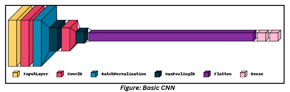
As shown above, we’ll use a Convolution layer, Batch Normalization and Max Pooling along with one Dense and Output layer. We perform flattening right before the dense layers.
CODING THE ARCHITECTURE USING TENSORFLOW FUNCTIONAL API
I’m using Tensorflow’s functional API to code this up. Why?
Tensorflow’s Sequential API allows me to create models by stacking them layerwise. While this is convenient in most cases and quite simple to understand, it doesn’t let me create models that reuse/share layers or have multiple inputs and outputs.
The Functional API makes layers reusable it’s easy to define multiple inputs and outputs. Our current architecture is too simple to notice the difference, but as start looking at more complex architectures, we’ll see how much it simplifies the process.
Talking about the differences in detail will require a dedicated blog but I have added some content in the reference section. Check them out if you’re interested!
The code is available here: https://github.com/MohanaRC/DL_demos_tensorflow/blob/14af6b248c44b3e2df055c2a4b8e5bf7baa3188e/Parameters%20Demo.ipynb
Don’t bother about the training details for now, just check out the code and the model summary for now.
THE CODE
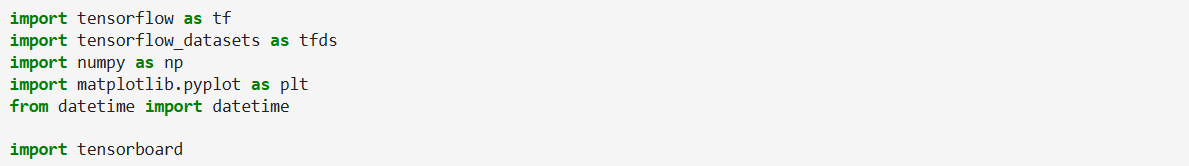
We’ll start by defining our packages,
Followed by defining all the layers,
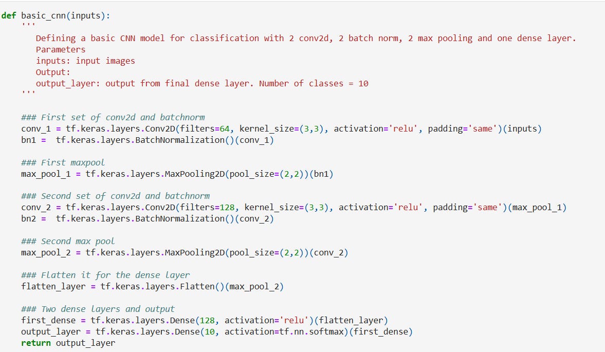
Notice how the layers have been defined. Since our model is very simple, the impact of using the Functional API isn’t very obvious. Fret not, we’ll talk about complex architectures pretty soon!
Let’s put our input and output together to create the overall model.
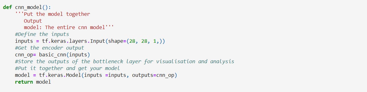

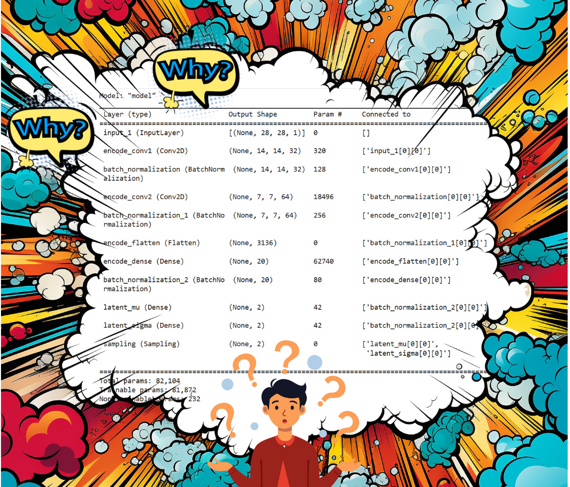
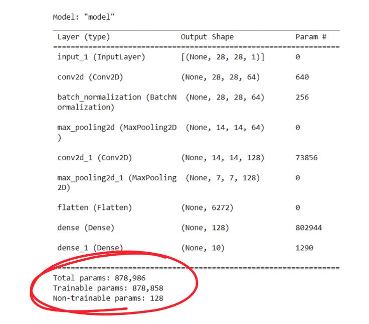
We have our basic CNN model! Let’s view the model summary,
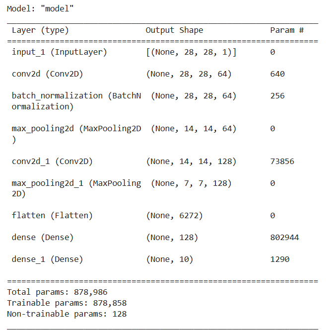
Check out the three columns- one for the layer type, another one called “Output Shape” which is nothing but the shape of a single output image/feature map. “Param #” indicates the number of parameters.
What are trainable parameters?
Trainable parameters refer to the parameters that can be learned and updated during the training process. Whenever we mention the term “training a mode”, we refer to these parameters. Pooling layers remain untouched during the training process, the activation function also remains unbothered.
What do we mean by output shape?
Output shape is just the dimension of the output feature map. What we see in model summary section is just the length and width of the output along a depth component that represents the number of filters that were applied to the input image. Think of it this way – you applied each filter to the input and received individual filtered images corresponding to each of the filters. One thing to note that the quantity mentioned in the model summary is very explicit to the same layer.
Let’s dissect each row in the model summary one by one.
LAYER 1: INPUT
This is just your grayscale input image of 28 x 28. Nothing for the model to learn here, so number of parameters is 0.
Notice the “None” everywhere in the model summary. This “None” indicates that the dimension is variable and will be updated based on the batch size assigned during the training process.
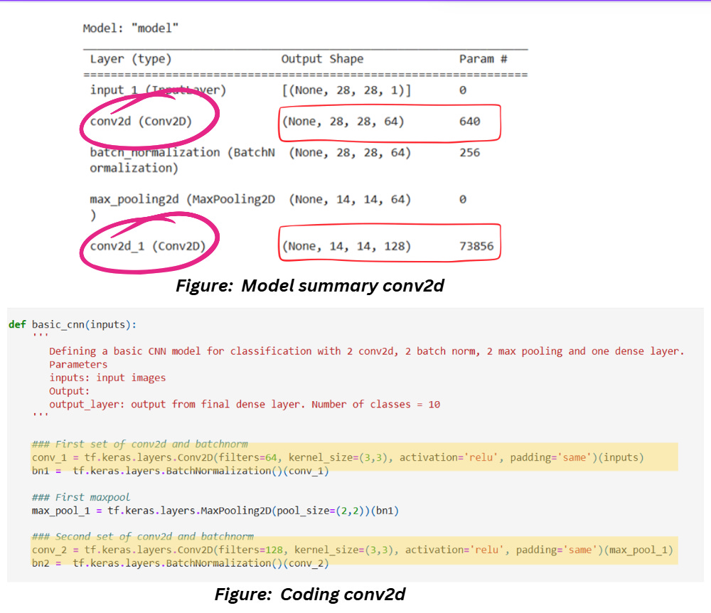
LAYER 2 AND LAYER 5: CONVOLUTION 2D
The conv2d layer is for applying convolution (and ReLU) to the images. We know that the kernels in the CNN layer will slide on the image, apply the filter and get the results as shown below,
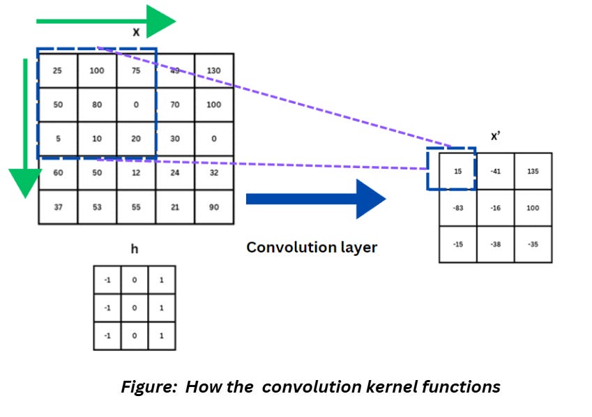
We also know that including a padding will add some additional pixels all around the image so that the kernel doesn’t start filtering from the edges directly. During the model training process, the values inside the kernel are tweaked, which means the kernel values are trainable parameters.
Output dimensions
The expression for calculating the output dimensions is given as follows,
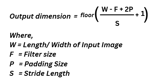
In CNNs it’s common to come across architectures that accept square images, so usually calculating this will give you the length and width of the images. If you’re using a rectangular image as an input, just calculate this separately for length and width. Kernels are usually square for convenience (they don’t have to be) but larger kernels have smaller output dimensions which justifies the minus. Adding a padding increases the output dimensions and the impact is on both edges of the images, hence the 2xP. Larger strides result in smaller outputs because we skip pixels based on this quantity, hence the division by S. The 1 in the end accounts for the initial position of the kernel.
Notice how the padding value has been set to “same” in the code. This indicates our output dimensions will be the same as the input except for the depth, which means a padding value is being assigned internally based on the other parameters (Stride and Filter Size). Curious about the padding value being set internally? Just substitute the values of the parameters as shown below,
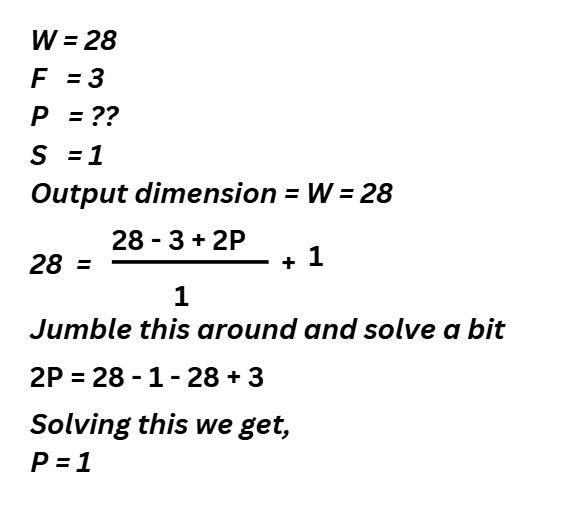
Substitute P = 1 in the expression for output dimension and you’ll get 28 as the output size.
What about the case when padding has been set to “same” but there’s a stride associated with this?
For example, check out the screenshot below,
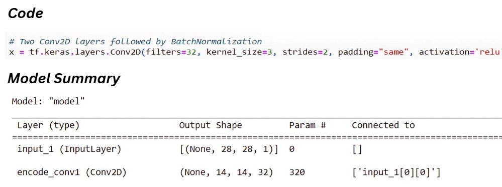
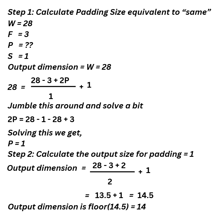
In cases like this, Tensorflow calculates the padding size first while considering the stride to be 1 and then recalculates the output size by substituting the calculated padding size, actual stride length and kernel size in the expression. Let’s have a look at the calculations for this,
Parameters
Parameters are dependent on 4 things – the size of the filter (which will be trained), the number of filters at the input (which determines how many trainable parameters we already had before) and the number of filters in the current layer (which determines how many we’ll add to the already existing inputs). And don’t forget the bias term which is just added to the end of this. The expression will look like this,
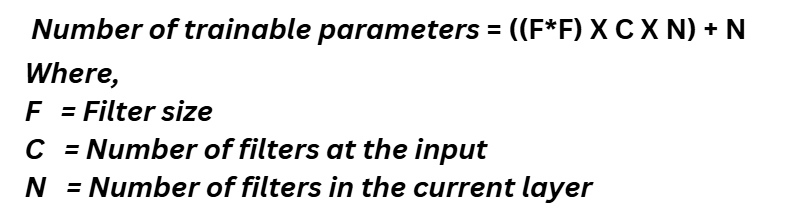
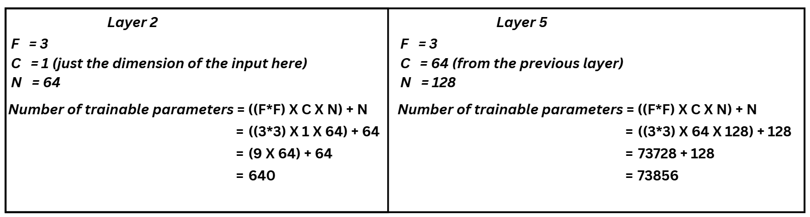
If the filters are rectangular, you can replace F2 by length x width of your filter. Let’s see this in action for the Layer 2 and Layer 5 which have conv2d kernels,
LAYER 3: BATCH NORMALIZATION
In a nutshell, batch normalization is a regularization technique that standardizes the inputs to the layer in a way that we have 0 mean and unit standard deviation. This in turn improves speed, performance and stability of the network.
Output Dimensions
Batch normalization doesn’t impact the dimensions of the image.
Parameters
Check out the image below,
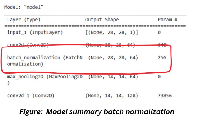
Where are the 256 parameters coming from? For this we have to dig deeper into batch normalization which I’ll cover in a separate article. But for now, let’s check out the mathematical expressions for batch normalization.
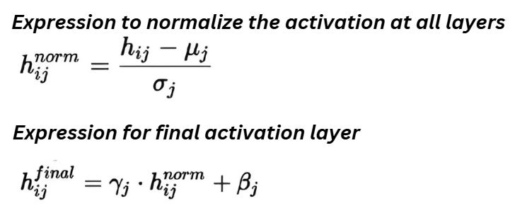
In the above expressions, µ and σ are mean and variance while ϒ and β are scale and shift parameters. These 4 parameters multiplied by the number of filters in our previous layer (64) gives us 4 x 64 = 256 parameters. Note that µ and σ are not trainable in Keras/Tensorflow so the number of trainable parameters is 128. You can validate this by checking out the bottom section of the model summary where the numbers for trainable and non-trainable parameters is mentioned specifically,
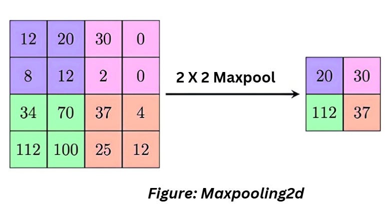
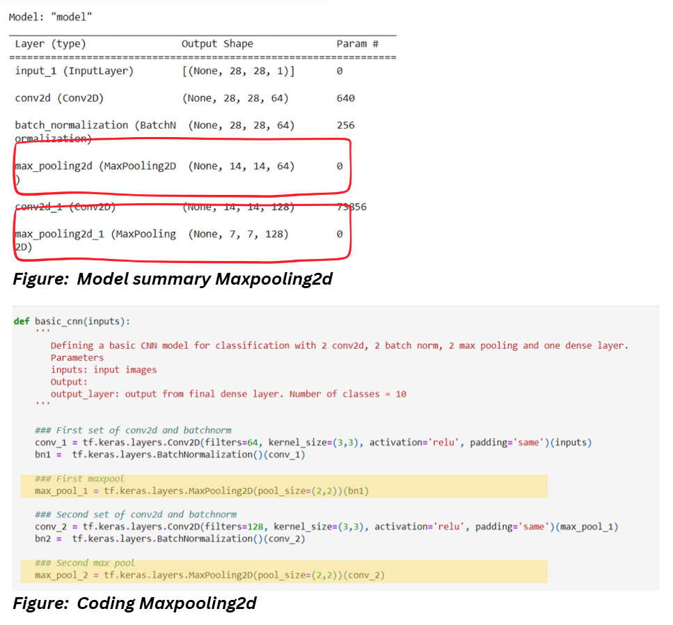
LAYER 4 AND LAYER 6: MAX POOLING
Max pooling is type of pooling operation that selects the maximum element a region of the image/feature map covered by the filter.
Check out the code and model summary section mentioned below,
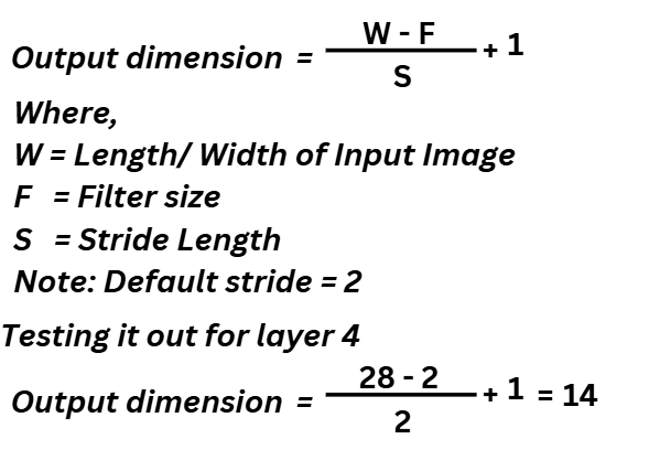
Output dimensions
The expression for output dimension along with the values for layer 4 is as follows,
Parameters
No filters or additional parameters involved in maxpooling. So, the number of parameters is 0.
LAYER 8 AND LAYER 9: DENSE AND OUTPUT
Dense layer is a type of layer in which each neuron from the previous layer is connected to each neuron of the current layer.
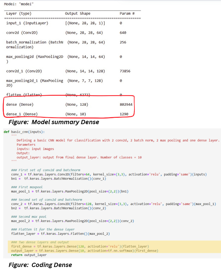
Output Dimensions
The output dimensions are already declared in the code. The second dense layer is the output layer so the output dimensions in a classification model is just the number of classes.
Parameters
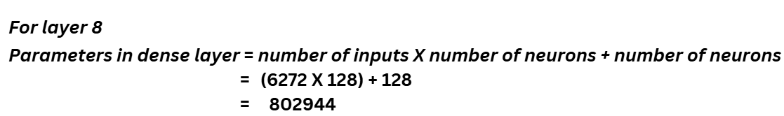
The dense layer follows the equation Y=WX+B where W is the weight matrix, B is the bias and X is the input to the layer (Note: A dot product is performed between W and X). The flatten layer in the step earlier flattens the images to 1D and that gives us the number of inputs X. The number of parameters is,
Parameters in dense layer = number of inputs X number of neurons + number of neurons
Let’s calculate this!
THE FINAL SECTION
We are talking about the section highlighted below,THE FINAL SECTION
We are talking about the section highlighted below,
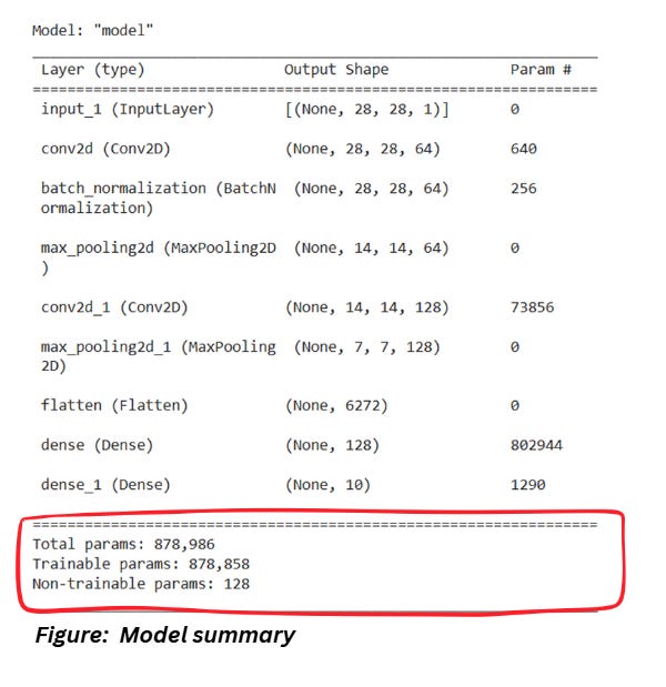
Nothing much here, just a sum of all the parameters and the sum excluding the non-trainable parameters in batch normalization.
REFERENCES
1) Sequential vs Functional Tensorflow: https://www.analyticsvidhya.com/blog/2021/07/understanding-sequential-vs-functional-api-in-keras/
2) Functional API Tensorflow documentation: https://www.tensorflow.org/guide/keras/functional_api
3) Batch normalization: https://medium.com/analytics-vidhya/everything-you-need-to-know-about-regularizer-eb477b0c82ba