


Everything you need to know about CNNs Part 8: Intuitively Interpreting the Loss Value & the Loss Curve
If you're training a machine learning model, the loss is everything. I mean EVERYTHING!


Welcome back to Part 8 of my series where we dismantle a Deep CNN completely and attempt to build it back layer by layer with of understanding how it works! Today we’ll try to make some sense out of the Loss computation process we discussed in Part 7.
Let’s have a look at the training process exactly like it was in Part 7 once again,

In today’s blog we’ll assumed we’ve covered all the stages in the feedforward direction and computed the loss value. Now the main question is …
WHAT DO WE DO WITH OUR LOSS VALUE?
The loss function we use gives us an estimate of how far our model is from the target value and interpreting this information properly is very important.

For instance, in Figure 2, Class1 is the clear winner with a distinctively higher score. However there could be a few alternative scenarios as well like the case were Class1 secures a majority with a score of 0.51, Class2 gets a score of 0.47 and Class3 and 4 have scores of 0.01. Here, Class1 is still the winner and matches the true label, but the competition is very close — a minor distortion in the input image might have switched the predictions!
If we don’t use a loss function to differentiate between the cases where the models predict the correct class with a strong confidence and when it can’t, we can’t really figure out if the model is really trained.
How do make sure that the correct classes are predicted confidently?
This is practically the job description of the final activation function and loss function!
The Softmax activation function blows up the differences in the logits. The Loss function blows up the difference in the performance. Think of these as a double check to make sure that even small differences are considered properly while training the model.
Now back to the question, what do we do with the computed loss?
The loss function quantifies the difference between the true and predicted labels. As our model predicts better, this gap between true and predicted labels should reduce. Which means as our model trains and learns how to extract the features according to the task, the computed loss should ideally keep decreasing as the model predicts the correct class with higher and higher confidence.
MODEL TRAINING AND LOSS VALUE
The model will output a confidence score during the training as well as the inference but the loss computation will happen explicitly in the training process
For training the model using the loss value, we use the following steps,
We check if the loss value is better or worse in the current iteration as compared to the previous iteration
Depending on point 1, we calculate the appropriate changes to the kernel values for the next iteration
Hope that our modifications in 2 land us with a lower loss value than the loss value in point 1
Repeat till we’ve either hit the lowest possible loss value, an early stop or completed all the epochs
Now you can see how loss computation is at the center of the training process.
Check out the loss curves in the figure below,
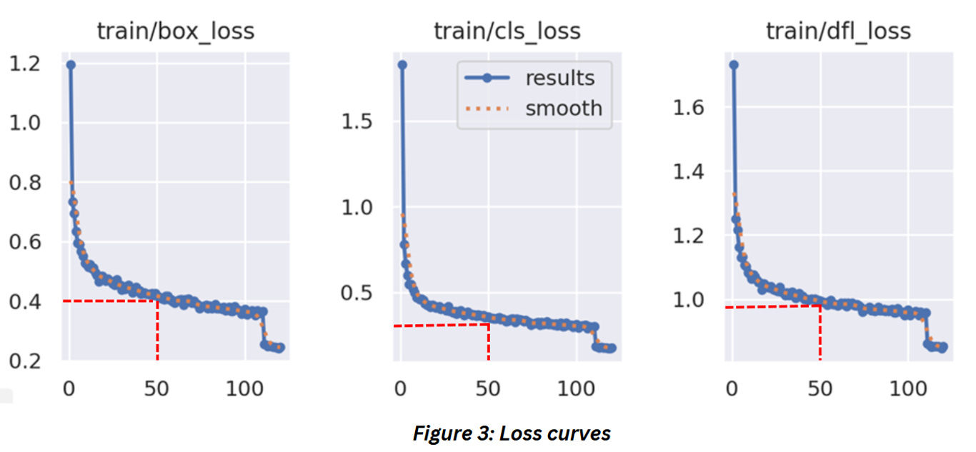
The x-axis of the curves represents the epoch and the y-axis represents the loss value of the model corresponding to that epoch. There’s a red dotted line marking the loss value at the 50th epoch for your reference. These models have been training for 150 epochs and use pretrained imagenet weights.
Don’t worry about the terms box_loss, cls_loss and dfl_loss now. These are loss values monitored during the training of a YOLO model which we won’t cover now. Consider these as generic examples for loss curves and use the concept to understand the training process of any model.
If you observe any (or all) of the curves you’ll probably notice that,
The loss values take a huge dip in the beginning of the training. This is pretty common, especially if you use initialize the model with pretrained weights. Assuming there are no issues like challenges with data etc. the model is able to adjust the weights pretty quick at this stage
Sometime after the initial epochs, the change in loss value appears to slow down gradually. This is expected as well — think of this as the model slowly learning to work on the tougher examples in the training data in the later epochs
Ideally the curve should be smooth like the orange line but that’s rarely the case. During the training, the model might make a couple of unwise weight adjustments here and there — it could be due to the batch, it could be something to do with the data or it could be a local minima (we’ll cover it right after this). Occasionally the loss might even appear to increase or “spike” a little here and it’s not that uncommon, especially with real world data that isn’t as clean as standard datasets
When the model reaches a point where it can no longer be trained (usually), you’ll notice that the curve becomes almost parallel to the x-axis. This plateauing of the curve is known as convergence. In figure 3 you can see the curve is still sloping downwards which means there’s probably scope for further training but in figure 4 below, you’ll notice how the training curve sort of flattens. This is the point we want to reach while training our model


ONCE WE HAVE THE LOSS VALUE, HOW DO WE DECIDE HOW TO CHANGE THE MODEL WEIGHTS
This is a massive topic which we’ll cover in the upcoming parts but let us have a quick overview.
The loss curves we’ve displayed in figure 3 and 4 are very simplified versions of the loss curve used for monitoring the training. Figure 5 shows an actually loss curve might look like,
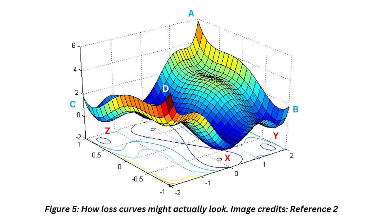
Complicated is one word for this!
Think of this curve as a solid sheet. Now imagine the process of loss minimization as placing the ball somewhere in the edge of the sheet and letting it roll downwards. In Figure 5, if I let a ball roll off point A, based on the slope and how we decide to move the ball, it might land in point X which does seem like the lowest point in this curve (and our best-case scenario). There’s another case where we keep rolling the ball slightly towards the right side and the ball lands in point Y which might look like the minimum but it is not. Which means ball will be stuck. Similarly if the ball starts from points B and C, the loss values might look good initially but we might get stuck in points Z and Y very quickly.
Points Y and Z are called local minima and if you are training a model on real world data you will definitely encounter them. Don’t worry, there are strategies to avoid and overcome them. In curves similar to figure 3, the local minima may appear as sections where the loss values appear to get stuck but it drops out of it after a handful of epochs. The objective of training a model is to find point X, which we’ll call the global minimum.
WHAT ARE THE FACTORS THAT IMPACT MODEL CONVERGENCE?
Let’s say we are all set on the model architecture. We know what layers we’ll use, we are set on the number of layers etc. This means our loss curve is set — every architecture has different loss curves based on the complexity, the layers etc. The moment we decide on the architecture, we have an approximate loss curve that we have to navigate for the particular dataset. This is also a reason why the selecting the right architecture can make a huge difference! You don’t need complicated state-of-the-art models for everything! The dataset and the model architecture will primarily determine the loss curve. There’s a third factor which is the batch size which we’ve covered a bit in Part 5 of this series.
Based on this, we can intuitively infer that the factors contributing to convergence, or finding the global minimum are,
At which point on the curve we start the training process
How we navigate the loss curve to find the global minimum
Where we start the training process is primarily determined by the initial weights, which is why its often a good idea to initialize the model with pretrained model weights. The shallow layers of the model will already be quite optimized (or will atleast optimize quickly) for higher level features and most of the training will focus around fine-tuning the weights. More details on this will be discussed in a separate blog.
In Part 9 of this series, we’ll discuss Optimizers which are very important to determine how we navigate across the loss curve and find the global minimum. Optimizers along with other factors such as learning rate, momentum, learning rate decay etc. determine how we move along the loss curve while avoiding and overcoming local minima during the training process.
REFERENCES
1) Diagnosing model curves: https://machinelearningmastery.com/learning-curves-for-diagnosing-machine-learning-model-performance/
2) Analytics Vidhya Loss functions blog: https://medium.com/analytics-vidhya/introduction-of-different-types-of-loss-functions-in-machine-learning-and-deep-learning-66ef7804668b
3) Deep Dive into loss curves: https://wandb.ai/mostafaibrahim17/ml-articles/reports/A-Deep-Dive-Into-Learning-Curves-in-Machine-Learning--Vmlldzo0NjA1ODY0