Everything you need to know about CNNs Part 3: Pooling Layer

Massive feature maps disrupting your model training process? Pooling layer to the rescue!

So far in the series, we’ve talked about the Convolution layer and ReLU (Link). Let’s move on to the second set of feature extraction layers in a CNN – the pooling layers. Check out Figure 1 to see where they’re placed in a CNN.

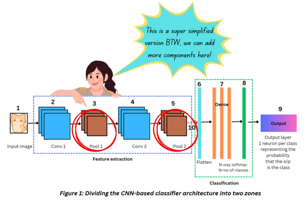
As shown in Figure 1, the pooling layer usually comes after the convolution layer (or better, convolution+ReLU). If we refer to the VGG16 architecture, pooling layer is placed like this,

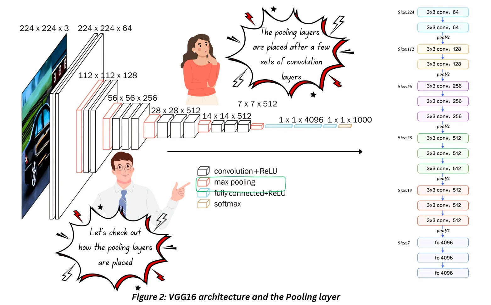
The pooling layer is placed after a few sets of convolution layers here. The architecture appears to have 3 sets of convolution layers back-to-back followed by a single pooling layer which cuts down the size of the output by half. The convolution layers are definitely using the parameter “same” for padding which ensures that the output dimensions don’t shrink after the operation. Now let’s talk about pooling and what it does.

POOLING LAYER

In CNNs, the pooling layer is inserted after the convolution layer and the activation function to downsample the output feature map. While downsampling a feature map will most definitely lead to some amount of data loss, the pooling layer is designed to retain the most relevant information from the feature map based on what type of pooling is used.

When there’s a concern about data loss, why perform pooling in the first place?

To answer this, let’s have a look at the model summary of VGG16 architecture.

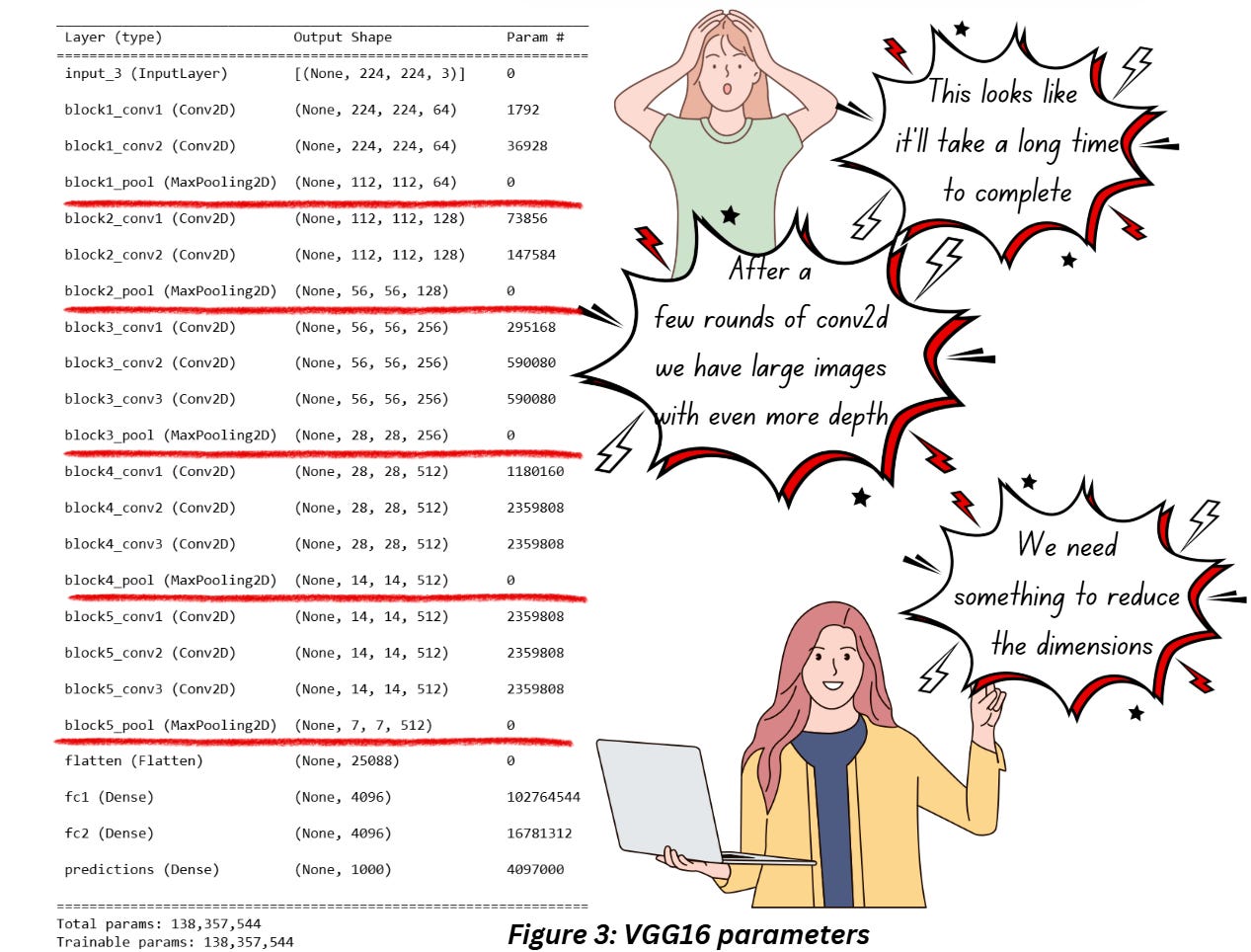
Check out what happens after a few rounds of conv2D. To prevent any information loss at the edges we’ve added a padding and retained the size of the image. But what we end up with is a large feature map with a much larger depth. In the following layer, we’ll have to perform the same set of operations on this feature map and this goes on and on. We don’t have unlimited compute - GPUs are expensive guys!

One way to tackle this would be to reduce the dimensions of the feature maps but we have to do it in a way that lets us retrain the most important aspects of the image — we still want to perform our classification task at the end of the day! That’s where pooling techniques come in handy. And don’t get me wrong — that’s not the only thing pooling does but we’ll talk about it in some time.

To understand how the layer output dimensions and parameters are calculated, check out my blog Between the Layers: Behind the Scenes of a Neural Network.

Note: We might have put pooling layer under the heading of the feature extraction but pooling layers don’t really extract features as much as they compress them!

TYPES OF POOLING

Max Pooling

We’ll start with the most popular option – max pooling. When it comes to pooling operations, the names are kind of self-explanatory. Max pooling involves using a filter to scan all over the image and return the maximum value from every region the filter scans over. Check out Figure 4 which shows how max pooling is performed,

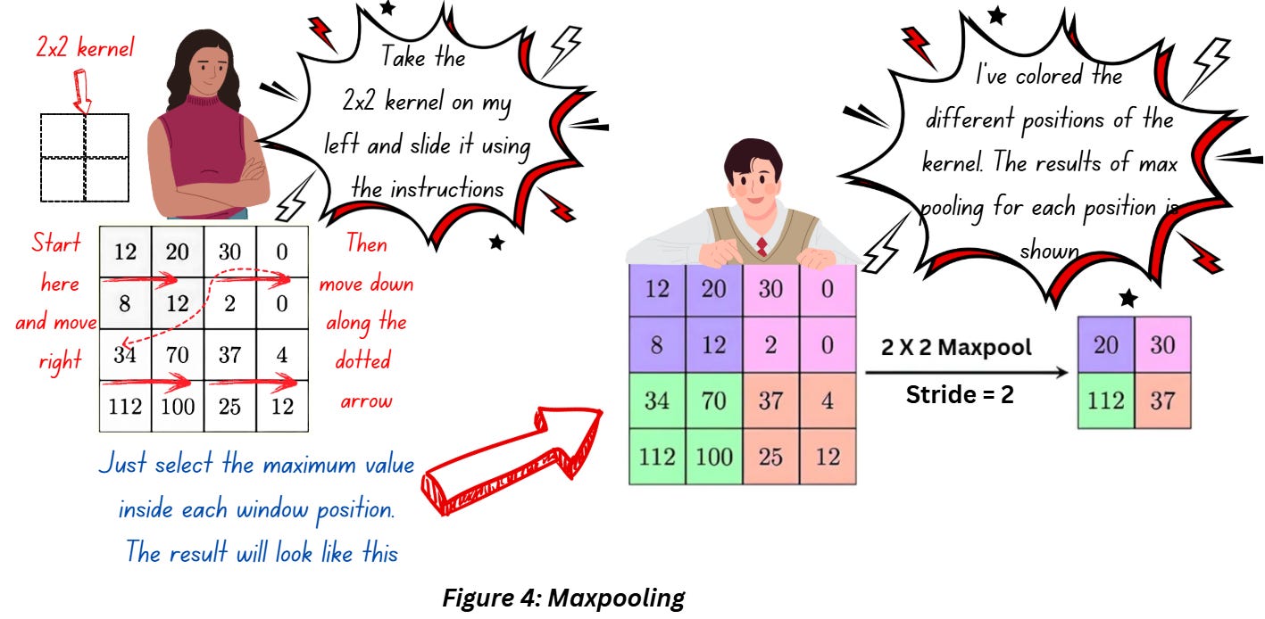
The kernel or the filter here is kind of like a window pointing at the region to focus on. We slide this kernel along the image as shown in the arrows, the stride is set to 2 so we are skipping a pixel between positions. In each position we just pick up the largest value (in the position marked by purple zone 20 is the highest value, in the position marked by pink 30 is the highest and so forth).

In essence, we’ve converted the 4x4 feature map to 2x2!

Why is max pooling so popular in CNNs?

Quite frankly I am yet to find a concrete reasoning behind this one. A lot of it is based on experimentation and empirical evidence. But intuitively, think of the largest values in a region as the most prominent features. In classical image processing, for techniques such as kernel-based edge detection, the large positive values would indicate the presence of an edge. The same logic can be used to justify the process of picking up the largest value in a region and preserving that for further processing.

Wait, so you’re telling me we’ve added a padding to preserve the size of the image in the feature map and then we add an additional layer to lose more information anyway? How does that make sense?

If you’re thinking we’ve already performed a similar process in the convolution layer, you’re right. You might also be thinking that we could reduce the dimensions of the output feature map by playing around with the kernel size and stride – and you’re right once again. But,

- Convolution is computationally expensive and compared to that max-pooling is a walk in the park. You have no trainable parameters or anything

- If don’t use padding you might lose essential information from the edges. Max pooling with all its flaws preserves the most dominant features

- Using a larger kernel or a larger stride makes the data loss a bit more uniform (like you skip every 1-2 pixels while moving along the image) but who’ll guarantee that you won’t end up losing some important information while making that skip? With max pooling unless you have massive kernel sizes and make massive strides (which you won’t if you’re building something serious) you will retrain whatever appears to be dominant in a particular window.,

Max pooling also introduces a little bit of invariance in terms of translation, shift, rotation, and scale which we’ll discuss in a separate blog under this series.

Average/Mean Pooling

Self-explanatory names, just use the average value instead of maximum and you’re good to go!

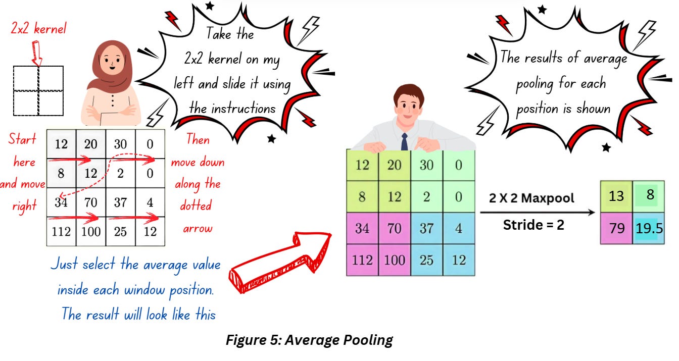
Average pooling has more of a smoothening effect and might result in the sharper features not getting identified. When it comes to retaining dominant features, it doesn’t have the same effect as max pooling.

Average pooling in its current form is not a popular component in CNNs.

FAQS FOR POOLING LAYER

Do I always need a pooling layer?

Not really, some architectures entirely skip pooling layers and use convolutions with a larger stride to downsample the image. Standard architectures usually have pooling layers.

What would be my ideal kernel size and stride?

I’ve usually seen 2x2 kernel size almost everywhere with a stride of 2. It halves the image and that should be enough reduction for 1 layer! Reference 6 mentions 3x3 kernels in the early layers of the CNN in order to reduce the size of the image quickly so unless you’re using huge images you won’t be needing that. Anything bigger than 4x4 will be counterproductive to our task as it’ll cause a massive amount of information loss. Downsampling is fine as long as we have enough information to perform our task!

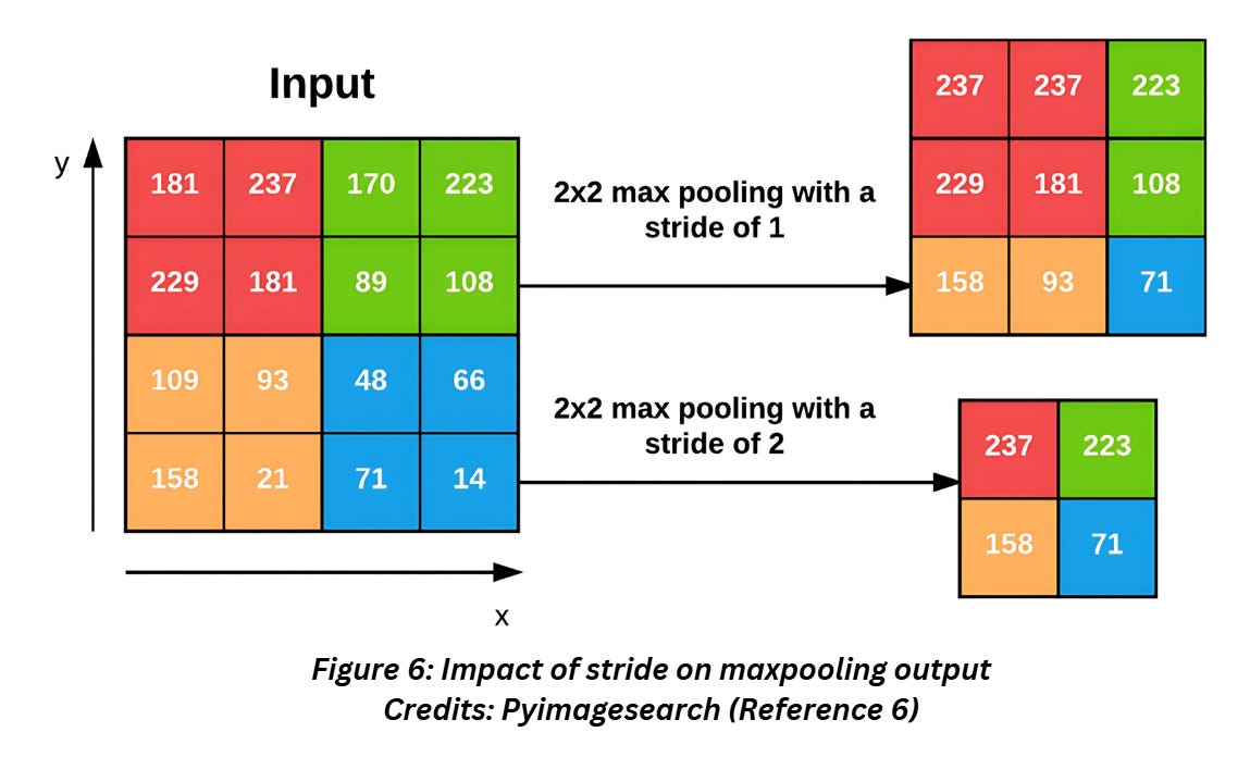
Can I use stride = 1 for pooling?

Yes, but it’s more common to use 2. If you use a stride of 1, the dimensions will not reduce as much as in 2. The image below shows the difference between the two.

OTHER VARIANTS

Max and average pooling might be the more common in the pooling layer but there are a handful of other pooling operations that might share the same name but have a different objective entirely. Here’s a list of them-

Global Average Pooling

Global Average pooling is an operation that can replace the fully connected layers in a CNN. While discussing the fully connected layers is beyond the scope (and the word limit) of this article, we’ll get to it later in the series. But to give some context, the fully connected layers are usually the last few layers in the CNNs and the result of this/these layers is fed directly to the softmax layer in a classification model – global average pooling is an alternative to this layer.

Functioning wise, global average pooling reduces each channel in the feature map with the average value of that channel. Basically, just take the average of the whole 2D and forget about kernels and strides!

Global Max Pooling

Similar to Global Average Pooling but select the maximum value of the channel instead using the average.

ROI Pooling

The Region of Interest Pooling or ROI pooling operation is very specific to object detection and semantic segmentation models so I’ll have to skip the details for now. In essence, it is used as an approach to extract small feature maps of a fixed size in Fast-RCNN. Features extracted from each of these regions is used for regression (to estimate the location of the object) and classification (to identify the object).

Stochastic Pooling

As the name suggests, stochastic pooling is a pooling operation that involves a probability distribution (pro tip – anytime you here stochastic, you can always assume there will be probability and stats involved in the process!).

Stochastic pooling operation is just like our regular max/average pooling but instead of being fixated on the maximum or average value, it selects a value based on the probability distribution derived from the values in the pooling region. Introducing some randomness in the process has an added advantage of functioning like a regularizer and avoiding over fitting!

REFERENCES

1) Pooling blog: https://machinelearningmastery.com/pooling-layers-for-convolutional-neural-networks/

2) Pooling and fully connected layer blog: https://brightonnkomo.medium.com/convolutional-neural-networks-part-4-the-pooling-and-fully-connected-layer-394ec01fb00d

3) Average pooling: https://www.sciencedirect.com/topics/computer-science/average-pooling

4) Global average pooling: https://paperswithcode.com/method/global-average-pooling

5) Stochastic pooling: https://medium.com/@crishna0401/stochastic-pooling-eda90d293ced

Pyimagesearch Convolution and layer types: https://pyimagesearch.com/2021/05/14/convolutional-neural-networks-cnns-and-layer-types/