
Everything you need to know about CNNs Part 1: Convolution Layer
Everything you'd ever need to know about the Convolution Layer in one place!

ZOOMED OUT INTRODUCTION
Since CNNs are a subset of Machine Learning, let’s stop and think about how a basic ML model would work for a relatively simple problem like classification.
To train the simplest possible classifier, on the data side we’d need
A dataset
Some ground truth labels for the training data
During the training process,
We’ll extract features
Pass the features to a model that will predict a label
Match the predictions with the ground truth
Quantify how far off the mark our predictions were from the ground truth labels
Use the information above to calculate a loss
Backpropagate the loss to tweak the parameters of the model
Repeat all the steps above till we conclude the training process (and hopefully learn to predict the correct labels)
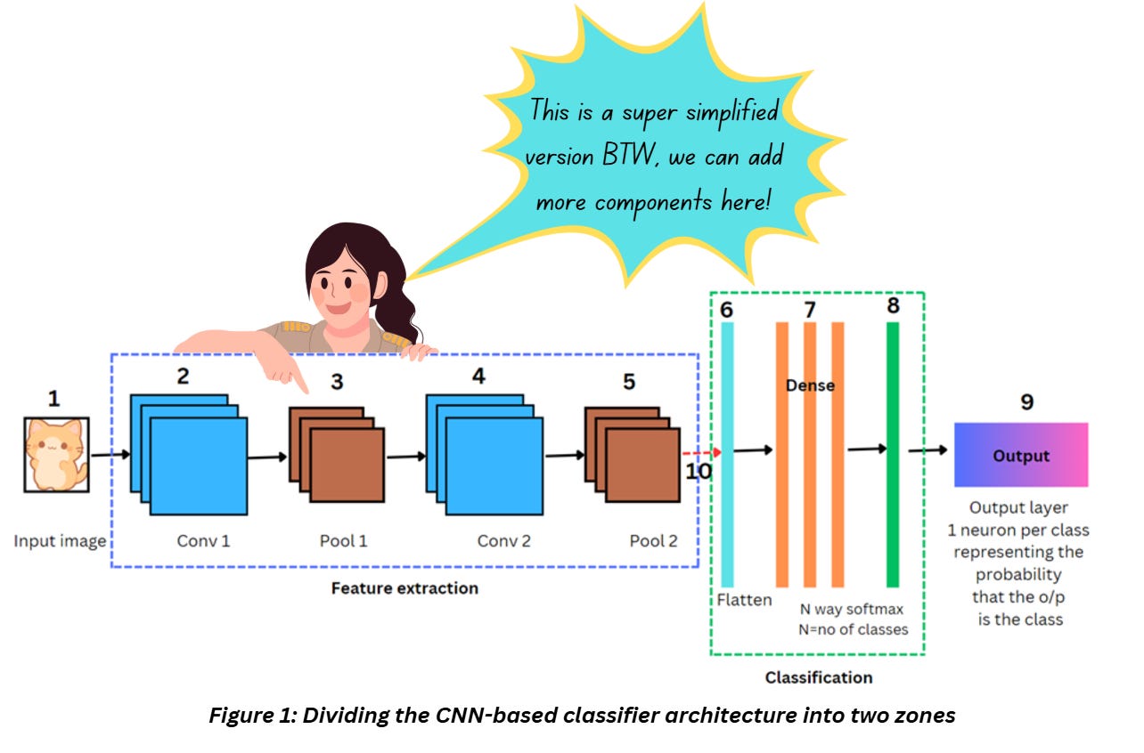
What I’ve mentioned above gives a generic idea about supervised learning irrespective of whether we choose a deep or not-so-deep network. Based on what we discussed so far, a generic CNN-based classifier (or any classifier for that matter) can be divided into two zones as shown in Figure 1,
The components I discuss in this series will all get plugged into one or more of the steps mentioned above.
CONVOLUTION LAYER
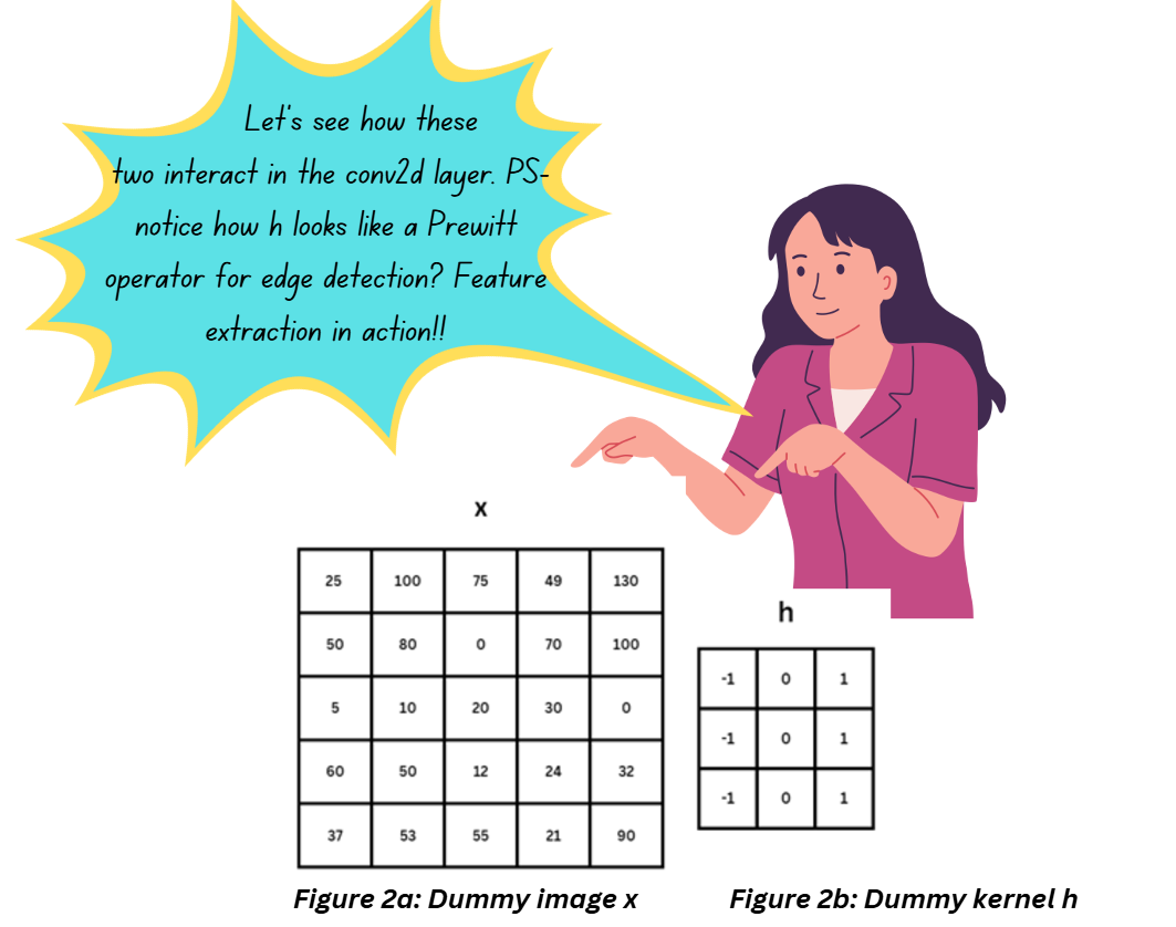
Even though the convolution layer is named after the convolution operation, it performs cross-correlation between the input image and kernel to produce the output. I’ve covered this in an older blog.
Let’s take a 2D dummy image x which we’ll assume to be the input of a conv2d layer. We’ll take a dummy kernel h which will slide along the image from left to right and top to bottom. The kernel weights will determine the features extracted from the image and are tweaked during the training process to ensure we extract the features we need to build a functional classifier.
It’s pretty common to have a large number of layers in a CNN where the shallow layers often extract features like edges and corners and the deeper layers detect high-level abstractions of the image (think of this as shapes and textures in a very abstract trippy format). We’ll need a separate article to explore that!
Let’s see what happens as kernel h slides along the image,
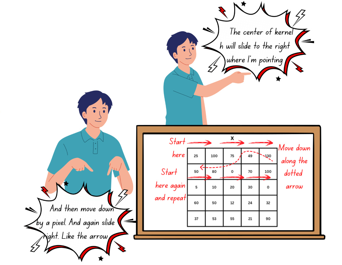
Inside the convolution layer, h will slide along the image x and perform an element-wise dot product at each position followed by addition to get the results, as shown below,
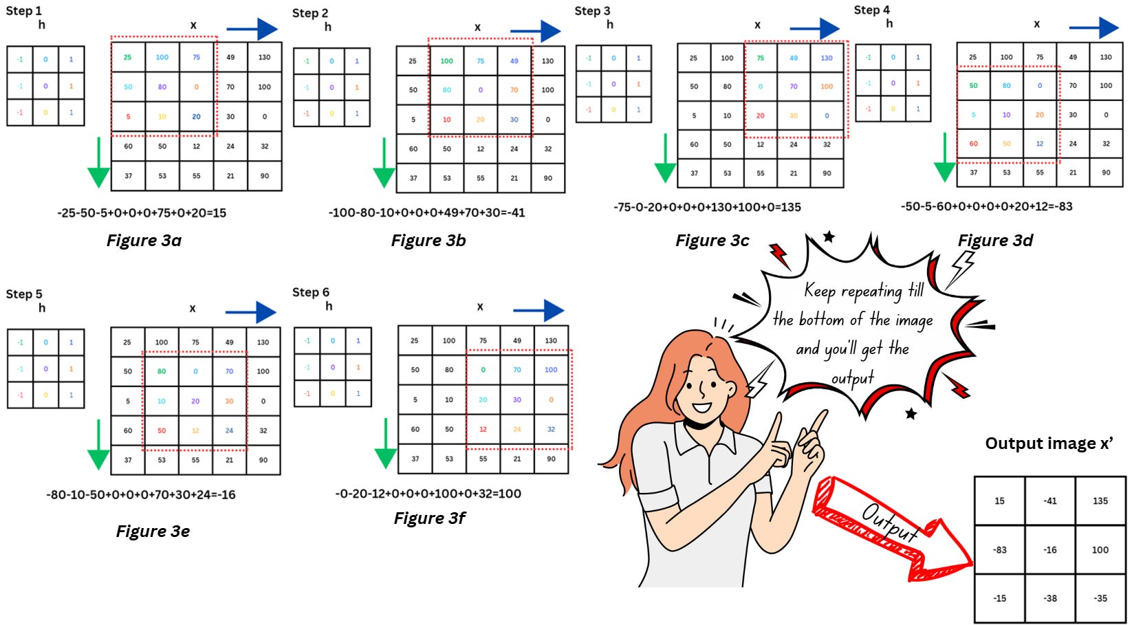
The output x’ is also another image consisting of the extracted features.
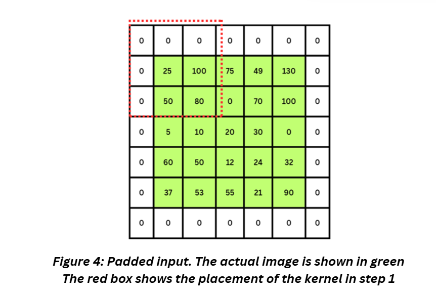
Notice that x’, is sized 3x3 while the original image x was 5x5, i.e., we’ve lost some information from the border pixels. One way to avoid this is by using a technique known as padding.
Padding
As we discussed, post conv2d layer we end up losing a slight amount of information from the edges. While it may not seem significant now, think about deep networks with stacks and stacks of layers – we will definitely end up losing a lot of information and some of it might be essential.
Padding expands the image just a bit to make sure that the image retains some of the information at the edges and the size of the image remains consistent. We do this by adding additional pixels at the border of the images.
There are a few types of padding and the difference lies in what we add in the edges. Some of the different padding strategies are Valid, Same, Causal, Constant, Reflection and Replication valid and same are the popular choices.
Valid padding in Tensorflow stands for no padding (like our example ealier). Same padding in Tensorflow requires a border of zeros to be added to the image and indicates that the output of the operation will have the same size as the input.
Stride
Stride in CNNs indicates if we will consider all the consecutive pixels in the image while moving the kernel or skip a step or two.
Let’s look at Figure 3a and 3b. Notice that the kernel has moved by one pixel from step 1 to step 2 – this indicates the stride is 1. If the stride was 2, the kernel would have skipped a pixel. Let’s add a padding to x and see how h moves when stride is set to 2.
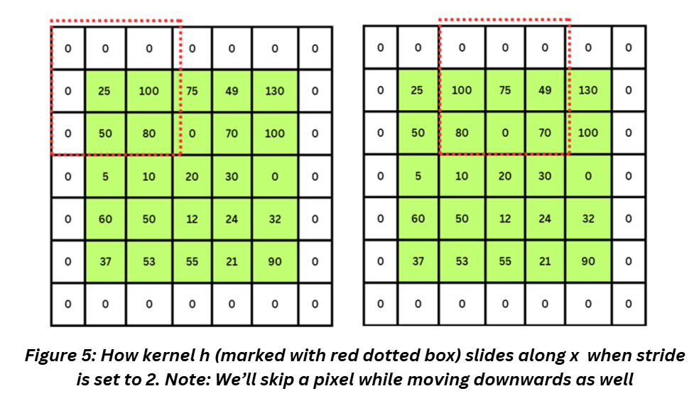
How does stride length impact the output size?
The output image will be smaller yet again. We stop losing information at the edges by adding the padding but we lose information inside the image when we use a larger stride.
How do we choose the stride?
There’s no right answer for this. Let’s say you have a large image and you’ll build your architecture from scratch. We’ll use the following image as example,
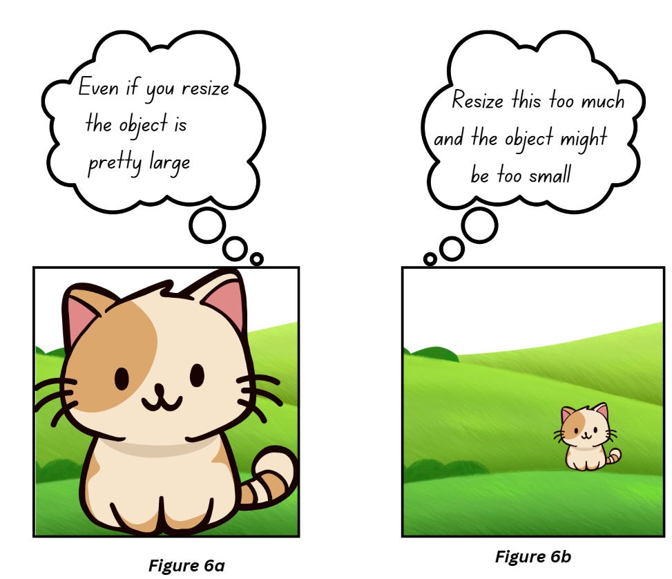
- Resize the image - Sweet and simple, but you might end up losing a lot of important information in the image especially if the object you are trying to classify doesn’t occupy a huge portion of the image (Figure 6b)
- If you use a larger stride and skip the initial resizing, you’ll get rid of some of the redundant information in consecutive pixels especially in cases when your object of interest has taking up most of the space in the image (Figure 6a)
- Using a larger kernel size might also be effective for Figure 6a.
By now it’s pretty obvious that increasing the stride reduces the size of the output feature map. What else does it do?
- Go back to Figure 3a and 3d, do you notice that the kernel operates on second column twice while computing the output? For Figure 6a, this can be a redundant bit of information. A larger stride can help with this. There’s a term for this redundant information – overlap of receptive field. Receptive field is shown in Figure 3 as the coloured pixels inside the kernel (formally speaking, it is the area of the input feature map that’s used to compute the output of a neuron).
- A larger stride length results in skipping some pixels while performing computations so we’ll be using less memory for the computation and our process will be faster.
- A larger stride might impact accuracy in cases like Figure 6b
KERNELS IN DETAIL
Kernels do the heavy lifting in the convolution layer – they’re practically performing a lot of the feature extraction. If this were a classical computer vision article, we’d have to discuss they’re types – different configurations of kernels extract different types of features like Pretwitt operator mentioned in figure 2. In CNNs is a bit straightforward because kernels because are updated during the training process.
Kernels are also called filters since they practically filter out information from the image. In general, they are small matrices which are moved around in the image to perform different operations and extract features. In classical computer vision, a kernel for smoothening the image would look different than a kernel for sharpening for example and the kernel weights will be predetermined. In CNNs these values are tweaked throughout the training process till we find the values that are the best ones for our requirement. When we talking about model learning, kernels are the components that “learn”.
If we consider one unit inside the convolution layer consisting of the region of interest in the input image, the kernel, and the output as a neuron, in a single layer we’ll have many neurons, each neuron will have a kernel that learns to pick up different information through the training process. A convolution layer will have multiple kernels stacked along the “depth”, each of these filters will focus on extracting specific kind of information from the image.
Go back to Figure 3 – coincidentally, the kernel h is the Prewitt operator for edge detection. As the training process progresses the Prewitt operator may or may not stay the same as the values of kernel start updating. Kernels are usually sized as 3x3, 5x5, 7x7 etc.
How do I choose kernel size?
- If you have a small sized input image and/or you want to extract minor/high frequency/small details form the image, go with a smaller kernel.
- If you have a large sized input image and/or you want to extract high level features and more distinctive details, go with a larger kernel. Larger kernels need a lot of padding if you want the output image to not shrink a lot
You don’t have to worry about the initial kernel values, that’s the model’s headache. You can initialize them with a constant value like zero or use a distribution but for standard architectures, you can just pick up a pretrained weights and update them during the training.
A larger kernel will downsample the image so if you wanted to downsize your image without resizing-resizing the image, going with a large kernel might be an option for you. Larger kernels will also make the network faster but you might miss out on the quality and quantity of features extracted which might impact accuracy. Again, no fixed rules, try out different combinations of kernel sizes, maybe larger kernels at the shallow levels and smaller ones in deeper etc.. An interesting activity could be going through architectures and seeing how the kernels selected.
1x1 kernels
You’ll see 1x1 kernels in popular architectures like GoogleNet, ResNet etc. but doesn’t really extract features. A convolution layer will have multiple such neurons and the number of neurons in that layer will determine the output parameters of that layer. Let’s say after a few layers like that we suddenly notice that we have far too many parameters and will need a lot of unnecessary computing power, we can use a 1x1 kernel to reduce the number of parameters without resizing the image but downsampling it along the channels (cross channel down sampling would be the fancy term for this).
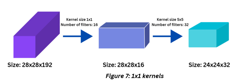
In figure 7, when the kernel size is 1x1, obviously there’s no change in the size of the image. But the number of kernels impact the depth of this feature-map, as in the number of individual feature outputs.
Can we use even sized kernels?
Every architecture seems to have odd sized kernels. Theoretically sure, we can use even sized kernels but using odd sized kernels simplifies our life.
For odd-sized filters, all the previous layer pixels would be symmetrically around the output pixel. Without this, we will have to have to deal with distortions that occur while using an even-sized kernel. With odd sized kernels, adding a padding to keep the dimensions of the output same as the input is quite easy. Simply put, it is easier to work with odd-sized kernels than even.
Note: Even though the terms kernel and filter are often used interchangeably, kernels refer to each individual kernel specifically, filter is the stacked up (concatenated) group of kernels.
To understand how the output sizes and trainable parameters are calculated, check out my previous article on the topic: Between the Layers: Behind the Scenes of a Neural Network
REFERENCES
Edge detection https://sbme-tutorials.github.io/2018/cv/notes/4_week4.html
Padding: https://deepai.org/machine-learning-glossary-and-terms/padding
Tensorflow masking and padding: https://www.tensorflow.org/guide/keras/understanding_masking_and_padding
Understanding valid and same padding: https://wandb.ai/krishamehta/seo/reports/Difference-Between-SAME-and-VALID-Padding-in-TensorFlow--VmlldzoxODkwMzE
Stride: https://deepai.org/machine-learning-glossary-and-terms/stride
Convolutions chapter: https://d2l.ai/chapter_convolutional-neural-networks/padding-and-strides.html