


THE OBJECTIVE
If the thought of going through derivation and theoretical examples gives you not-so-pleasant flashbacks from math class in school and college, I’m right there with you. I’ve felt the same way. I disliked sitting through classes where the professors would explain theory, I hated working on the derivations and I absolutely hated the practise of mugging them up for exams.
When I started working with Computer Vision algorithms, for more complex problems that couldn’t be solved with a pip-install or git clone I had to go through papers hoping to reproduce what was written in it. And let me tell you this I was colossally stuck on more than a handful of occasions.
The one way to get unstuck was to read math books and math theory; and get comfortable with the language used. Mathematical terminology is tough and if you’re not used to the language, you will get stuck over and over and the only way to overcome the challenge is by exposing yourself to the language over and over.
Another benefit of going through proofs and equations is gaining a well-rounded view of the final expression. If you are comfortable with the different steps in reaching the final expression, it’ll make you more comfortable in the application process. As we go through the math behind some complex algorithms in the later articles, you’ll observe how theorems have been seemingly inserted in stages where it’s anything but obvious. And you can only do that if you know what you’re dealing with in and out.
Enough lecture, let’s begin now.
THE PROOF
In the previous article (Link: Introduction to Bayes Theorem ) I introduced Bayes Theorem and talked about two different ways of writing the Bayes theorem:
Version 1:
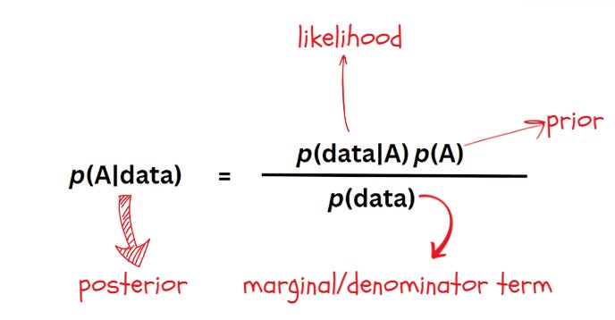
This is the usual way of writing the Bayes theorem and intuitively, this interprets the posterior as a combination of information from the past events combined with the information from the observed data. This is what we’ll be dealing with most of the time. Let’s also call this expression Equation 1.
Version 2:
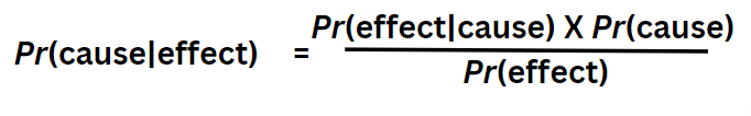
In this version, the posterior is expressed by describing the events in terms of cause and effect. Let’s name this Equation 2.
Simple and Straightforward derivation of Bayes Theorem using conditional probability
For a quick revision, check out my older article describing Conditional Probability and other mathematical terms that will come in handy as we derive Bayes Theorem (Link: Introducing the Basic Terminologies in Probability and Statistics)
Now let’s begin.
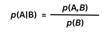
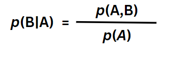
We know that for two events A and B, the expression for computing the conditional probability of A can be expressed as,

Let’s call this Equation 3a.
This expression computes the probability of event A occuring when it has already been confirmed that event B has occurred.
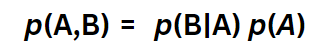
If I want to rewrite this expression for the event where B occurs after it has been confirmed that A has already occurred, the expression above can be tweaked a little bit and it’ll look like this,
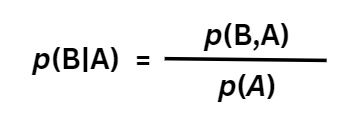
Let’s call this Equation 3b.
In Equation 3a and 3b, p(A,B) and p(B,A) are the probability of both of the events happening and they’re actually the same quantities but represented a bit differently (and in order). Why?
Let’s say you’re out for lunch date and you’re deciding what to order. Event A is you ordering a pizza and event B is your date ordering an ice cream. Now event A given B is the case where you order a pizza after your date has already ordered an ice cream. Event B given A is the case where your date orders an ice cream after you’ve ordered a pizza. If A and B are independent events, i.e. you ordering a pizza and your date ordering ice cream (and vice versa) have absolutely no relation (i.e. you were already in the mood for those particular items irrespective of what the other person’s order) then it’s just the same thing in a different sequence. This means p(A,B) and p(B,A) are the same quantities.
Going back to the equations, how about we maintain some consistency and rewrite both of them as p(A,B)?
This will now give us the two following expressions,
We’ll call this one Equation 3c. It’s the same as Equation 3a but just for continuity and easier reference, I’m putting it here.
And this Equation 3d
We’ll rearrange Equation 3d just a little bit.
And call it Equation 3e
We are set to substitute Equation 3e in Equation 3a to replace the joint probability term,
And we’ve finally derived the Bayers rule. Going to name it Equation 3f.
If we replace the events As and Bs with the terms “data” and “event”, “cause” and “effect”, the expression still remains the same. Now notice what happens when I jumble Equation 3f a little bit more,
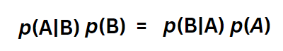
We’ll name this one Equation 3g. Intuitively it makes sense– whether you order a pizza after your date orders an ice cream or vice versa, you end up getting both pizza and ice cream and that is what joint probability quantifies as well. Pretty neat!
All this talk about pizza and ice cream, now I need to order one of them – can’t do both- too many carbs. Why are carbs so delicious, sigh!
Moving on to the example now!
The example

We’ll get into some calculations now so I hope you’re comfortable with the basics of Bayesian Statistics. The objective of this example is to get comfortable with the application side of the concepts. While this example might not be directly related to AI/ML, but problems like these will definitely help in solidifying your concepts and will come very handy when we start exploring probabilistic networks.
Time to play the game!
“I want to play a game” for this example. I’ll give you a box with five cards inside – the cards can be black or red. Don’t bother about the shapes, we are only concerned with the colours of the cards.
Now, I want you to pull one card out, any one – oh you picked a black card! Cool. Can you use this information to estimate the number of black cards in the box?
You’re probably thinking “I’m not a psychic, how can I tell!”, but you can actually use Bayes Theorem to solve this problem.
The assumption
To simplify this problem, we’ll assume a case where all combinations of black and red cards are equally likely.
The prior
Think about it, what is your prior? We know that prior is our belief prior to data collection. You can’t see what you’re picking up so you’re equally likely to pick up any of the cards. This means your prior probability is 1/6.
The likelihood
Let’s list down the 6 different possible combinations of cards that might be present inside the box.
- Case 0: No black, all red
- Case 1: One black, four red
- Case 2: Two black, three red
- Case 3: Three black, two red
- Case 4: Four black, one red
- Case 5: Five black, no red
Case 0 might sound weird but the name kind of makes sense because we’ve already established that you picked up a black card so the case with all red cards is impossible.
Let’s express this mathematically. A simple way to write the likelihood would be,
Pr(X=1|Y=α)=α/5
We’ll call this Equation 4. In this context we’ll read this as “probability that one black card was picked given the number of black cards is α”. Based on the 6 possible combinations listed earlier, we can say α Є {0,1,2,3,4,5}, i.e., α is one of the 6 values.
The marginal
We’ve arrived at the trickiest part of the solution now. We need p(data) to calculate our posterior. What is data and how do we compute the marginal p(data) or Pr(data)?
The only observation we have so far is you picking up a black card. Pr(X=1) is the same as Pr(data). We know that the denominator term or the marginal termed Pr(data) represents our probability over all possible data samples. Using this information, we know Pr(X=1) is only possible between Case 1 to Case 5. This indicates that our observed data will be the possibility that we pick up 1 black card in any of these cases. Using this information, we calculate the marginal term as follows,
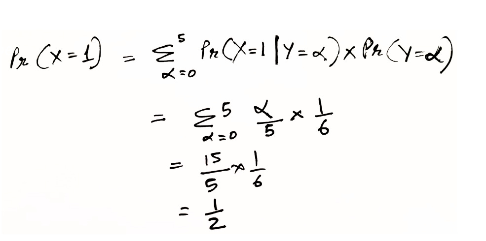
So, Pr(data)=1/2
The final steps
We have all the information needed to update the posterior. Let’s calculate the posterior and put it all together in a tabular format for all of the six cases.
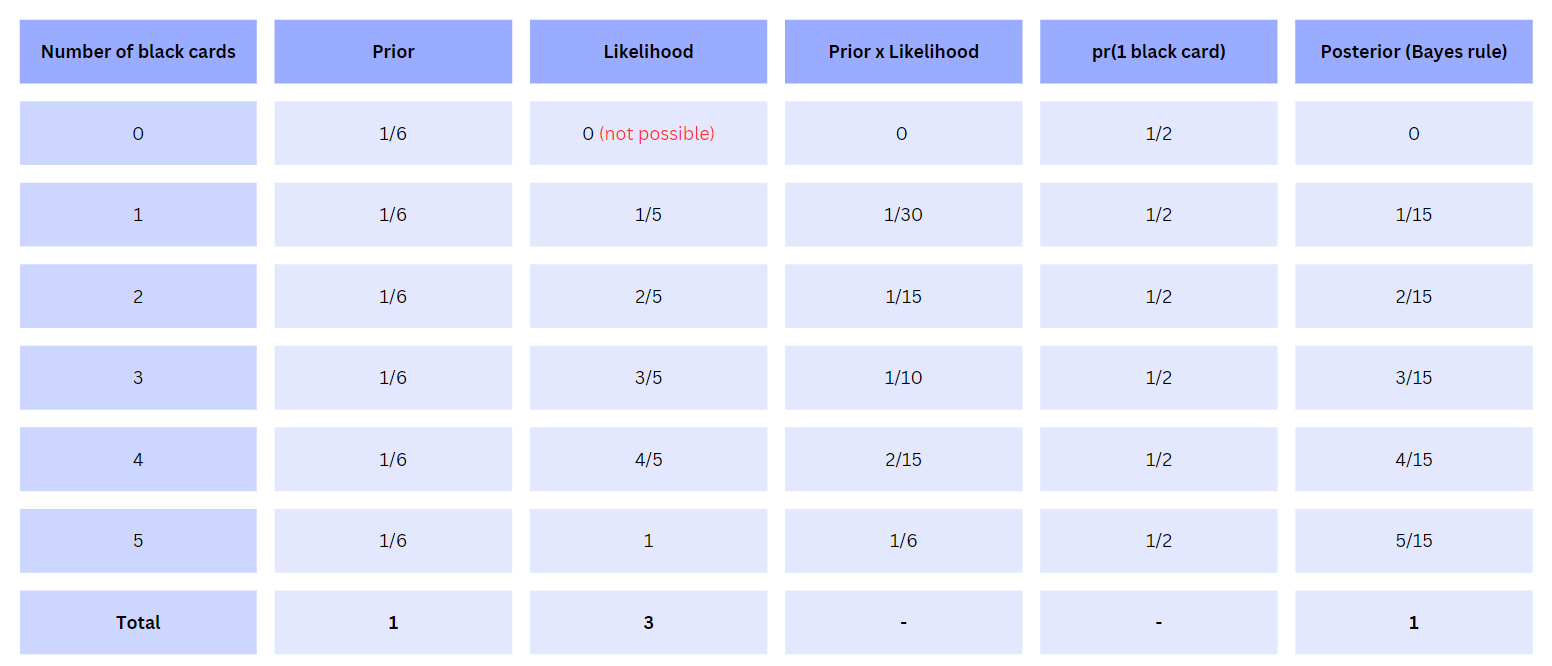
Table: Posterior calculated for the different combinations of cards (Reference 3)
Finally, we have the posterior values which estimates how many black cards we might have in the box based on the observation of picking up 1 black card.
I admit this isn’t as cool as I marketed it to be but trust me in the next few articles we’ll see how the humble Bayes Theorem is one of the most powerful mathematical concepts we’ve have out there.
References:
1) Classification of mathematical models: https://medium.com/engineering-approach/classification-of-mathematical-models-270a05fcac4f
2) Introduction to probability theory and its applications by William Feller: https://bitcoinwords.github.io/assets/papers/an-introduction-to-probability-theory-and-its-applications.pdf
3) A student’s guide to Bayesian statistics by Ben Lambert: https://ben-lambert.com/a-students-guide-to-bayesian-statistics/
4) Frequentist vs Bayesian approach in Linear regression: https://fse.studenttheses.ub.rug.nl/25314/1/bMATH_2021_KolkmanODJ.pdf
5) Mathematics for Bayesian Networks – Part 1, Introducing the Basic Terminologies in Probability and Statistics: https://mohanarc.substack.com/p/mathematics-for-bayesian-networks
6) Mathematics for Bayesian Networks – Part 2, Introduction to Bayes Theorem: https://mohanarc.substack.com/p/mathematics-for-bayesian-networks-3d1