
All you need to know about Variational Autoencoders
Simple, easy to grasp and detailed article on one of the popular Generative AI algorithms!

A light-hearted introduction
Once upon a time there was a model called Autoencoder. Autoencoder was a pretty handy dude, he was simple to construct and understand, he could perform a of tasks like image denoising, image compression, feature extraction and dimensionality reduction. Known to be a great image reconstructor, he could dump unnecessary details and store images in a small space and recreate a close version of it anytime. It was all going well till people started demanding more, reconstruction became backdated and generative models were the talk of the town.
Autoencoder had been around for a while and he was fairly capable of handling complicated tasks. He could stack up some “weights” for complex denoising work, throw in some convolutions to handle local context in images but by no means he could generate images. This changed on one chilly evening.
The year was 2013 and autoencoder was out on his regular retraining run. He was running, halting to check his stats and assess his training performance but he just couldn’t get his mind focused. He’d sprint for a while and suddenly he’d start panicking about his lack of generational capabilities. “What if they don’t want me anymore, what if I get shelved and people talk about me like I’m some legacy algorithm”, he kept muttering this over and over to himself. At one point he just stopped to contemplate if he should just give up.
All of a sudden, he heard a shuffling noise in front of him. It was a chilly December evening and through the fog he could see a man dressed in a suit standing right in front. He was standing in front of a carriage that looked like something straight out of the 50s. There was sudden a gush of wind and the man disappeared in the dense fog, where he stood lay a box.
Out of curiosity autoencoder walked forward and saw a note on top of the box saying “Drink up and you’ll be ready for the new era”.
Autoencoder was creeped out but desperate to stay relevant. He opened the box and found a tube with a blue glowing liquid. He took a deep breath and opened the cap, blue vapours and a nasty smell filled the air in front of him and before he could change his mind, he just chugged the whole drink in one gulp.
Immediately he started feeling his architecture cracking and expanding. The excruciating pain was something like he had never felt before and he knew something had happened. He immediately began a new training run. The was something was different this time, something complex had been added to his internal workings. By time he could get to the test run, he noticed that he was not just reconstructing his training images but he was actively modifying them. What sorcery was this?
I just told you guys a story that’s commonly whispered in AI/ML circles about the origin of VAEs. I’m no chemistry expert but I was told the tube with that blue liquid was spiked with Bayes Theorem. What I can tell you is what structural modifications happened to autoencoder turned him into a generative algorithm.
If you don’t know who autoencoder is and what he does for a living check out my blog on Autoencoders (Link: https://open.substack.com/pub/mohanarc/p/diving-headfirst-into-autoencoders?r=1ljeoy&utm_campaign=post&utm_medium=web )
AUTOENCODER VS VARIATIONAL AUTOENCODER
Autoencoders learn to extract dense representations from the input data and reconstruct the input image. The model has two components:
- The encoder which maps the input to a lower-dimensional format (latent space)
- The decoder which reconstructs the original input by mapping the lower-dimensional format to the original input format.
The output of the decoder is often a lossy version of the input image which is similar but not identical to the input because of the information loss during the process.
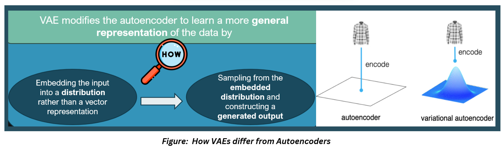
VAEs still do this, but the architecture has been modified to allow the model to learn more general representations of the training data. How?
- By using the encoder to embed the input into distribution rather than a vector representation
- Using the decoder to sample from that embedded distribution and construct a generated output
This process of embedding the input into a distribution and sampling from it to generate the output adds a probabilistic component to our model which allows the model to “generate” new samples!
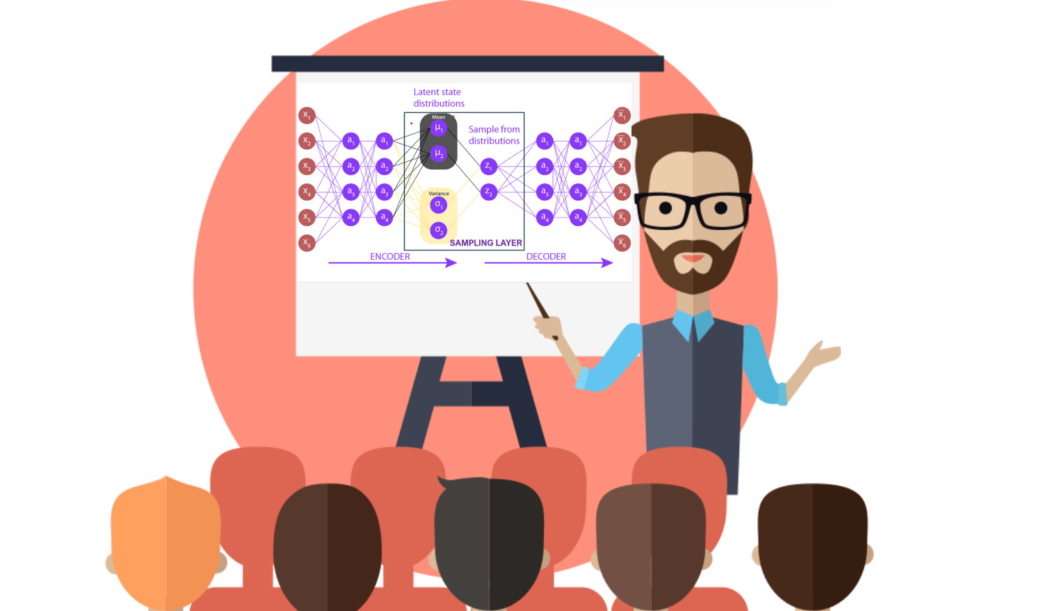
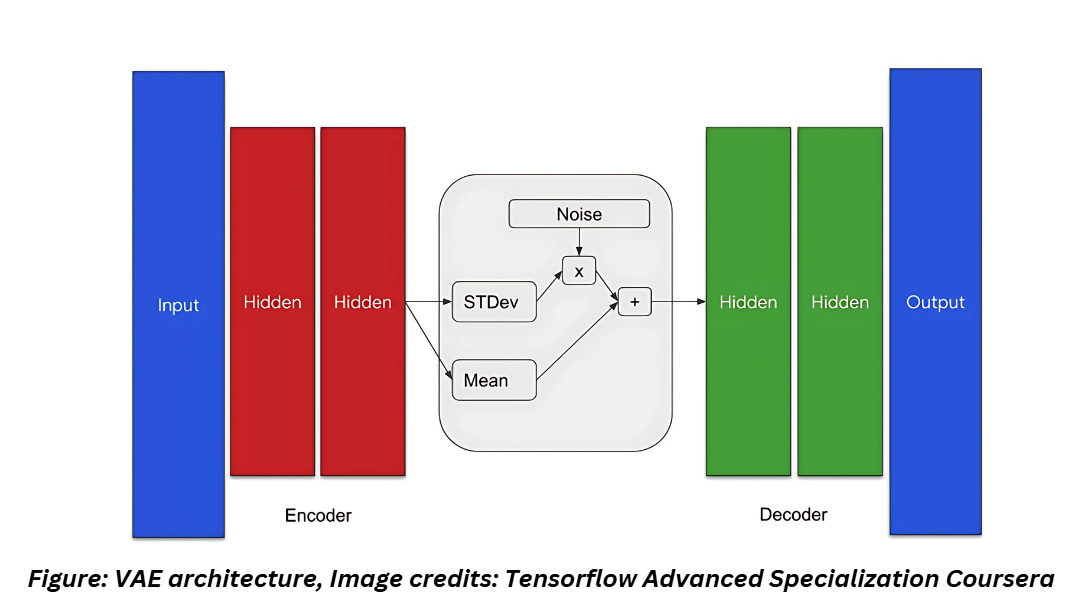
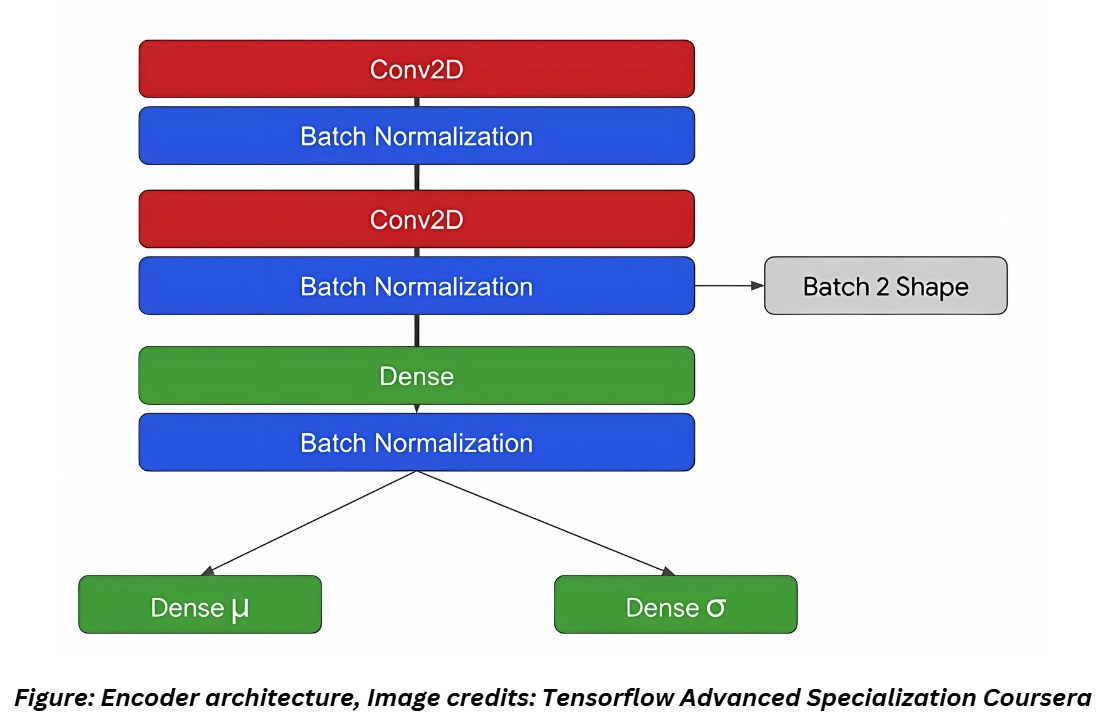
ANATOMY OF A VAE
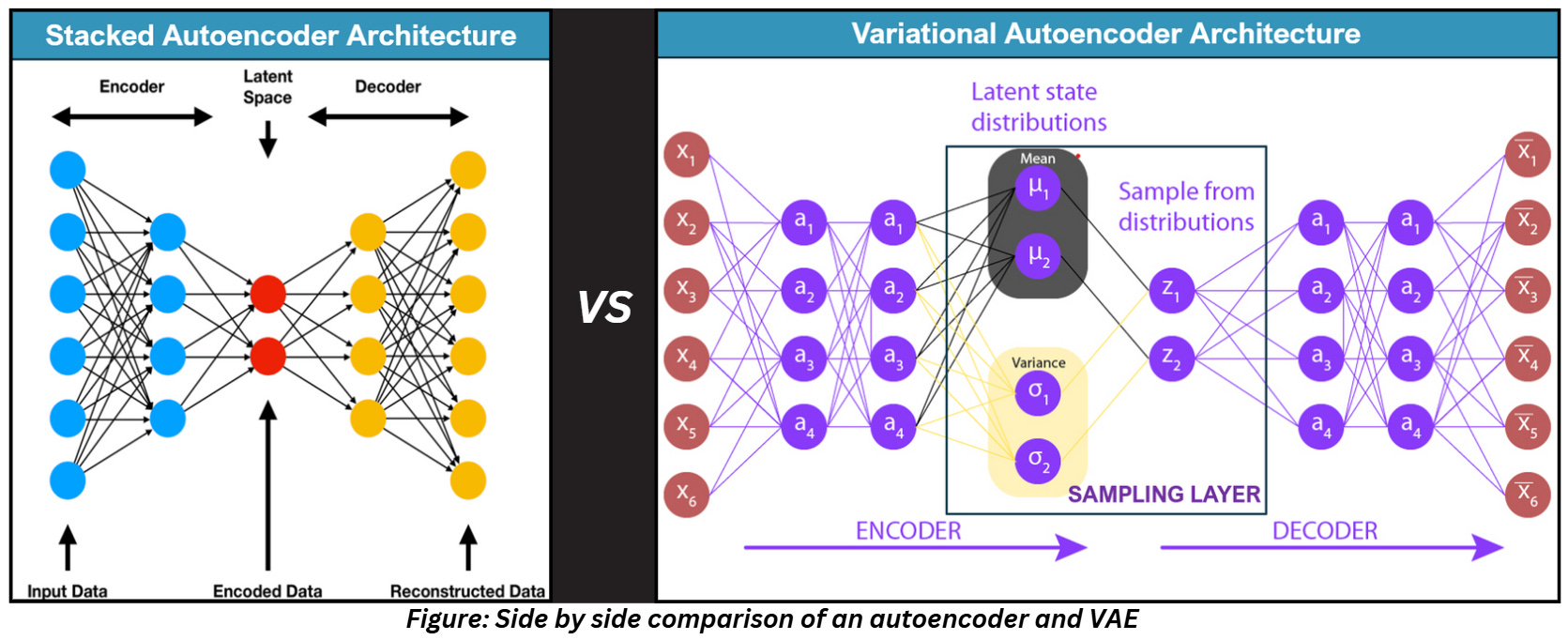
From the above figure, it is obvious what changed in VAEs. The encoder has two outputs in VAEs- the mean of the encoding and the variance of the encoding.
HOW DO WE USE THE MEAN AND VARIANCE?
The math of VAEs is far too complicated to be included in one article so I’ve written a separate one just for it (Link: https://open.substack.com/pub/mohanarc/p/applications-of-bayes-theorem-kl?r=1ljeoy&utm_campaign=post&utm_medium=web )
Just like autoencoders, we use the training images as target images while training VAEs. However, unlike autoencoders we don’t want the model to create a lossy replica of the input, so we need to find a way to construct a latent space that captures the essence of the input with some flexibility to create variations during the decoding process. That’s where the concept of using a distribution to define the latent space comes in. During the training process we find a way to create the ideal distribution for the latent space given our observation (i.e. our target which is just our input image).
We use a Gaussian distribution because it’s straightforward to implement with just the mean and the variance, it is a smooth distribution that prevents overfitting (so in a way it acts as a regularization mechanism as well!) and ensures small changes in the latent coordinates don’t cause abrupt changes in generated data.
If you go through my previous article on the math of VAEs, you’ll realize that we use KL-divergence and ELBO as a proxy to approximate the distribution of our latent space because we have limited knowledge of marginal term (if you need some help with basic stats, check out my series on these topics, link in the reference section).
Let’s get started with the code and we’ll discuss in detail line by line.
CODING VAE FROM SCRATCH
Let’s start by importing the packages and defining the parameters,
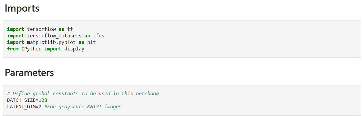
Latent Dimension
The latent dimension define above is the size of the vector that represents the compressed version of the input data in the VAE. This affects how much information the VAE can encode and decode, and how diverse the generated outputs can be. A larger latent dimension can capture more details and variations, but it can also lead to instability while a smaller latent dimension can force the VAE to learn more efficient representations, but it can also limit the expressiveness and quality of the outputs
There’s no specific process for selecting the optimal dimension, just experiment and compare the performance of the model and pick what suits the best.
Now we’ll prepare the data,
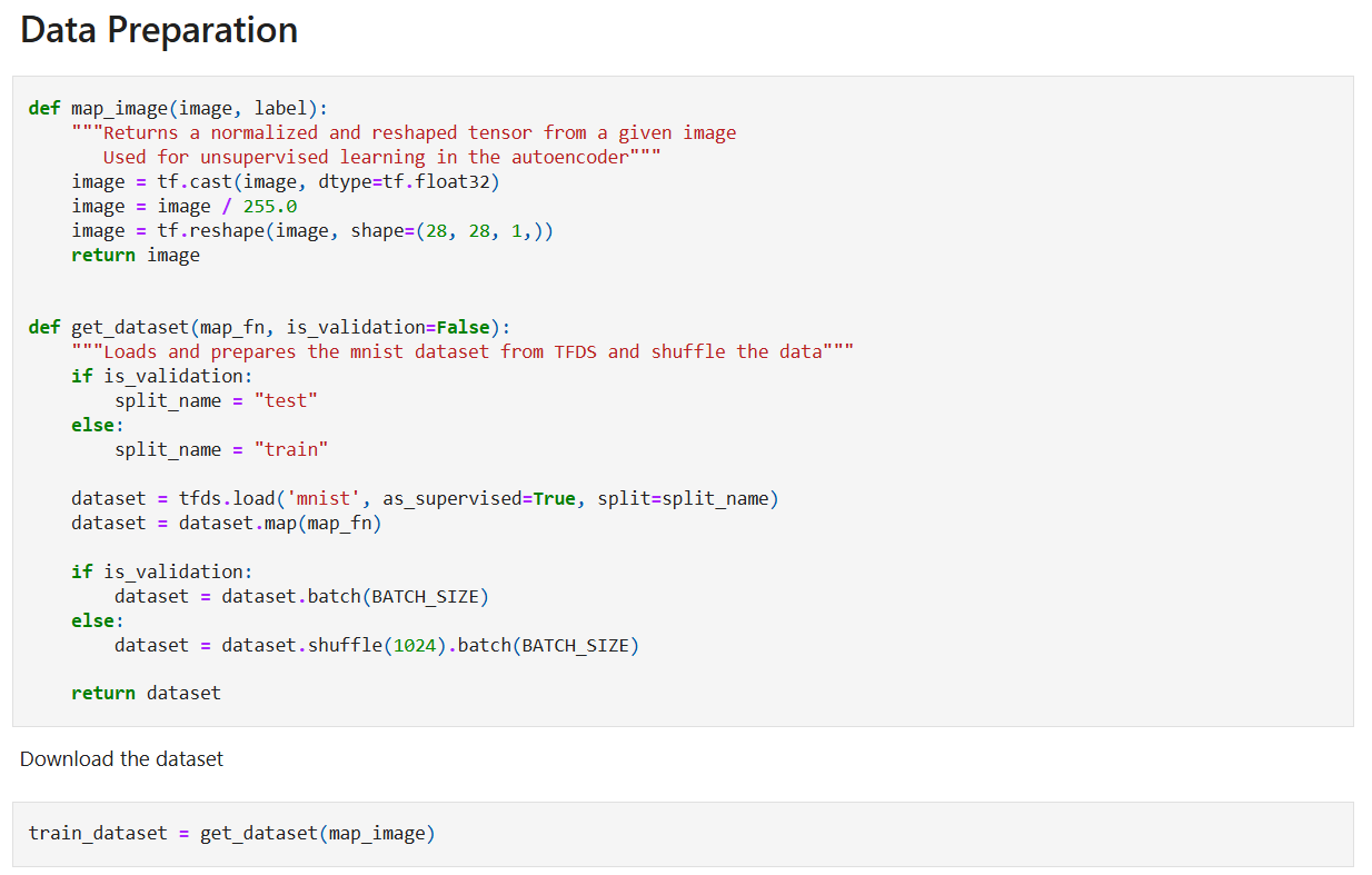
We are using MNIST dataset here so we’ll have to download, split, normalize and divide it into batches. Normalizing images improves performance by standardizing the images a little more.
Let’s start building the model now.
VAE components
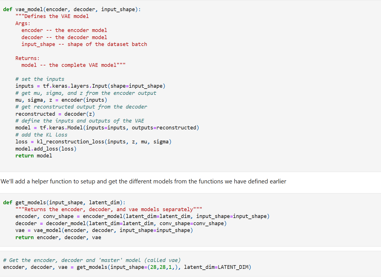
Our VAE model consists of three components —
The encoder: The encoder takes the raw data and transforms it into to a probability distribution within the latent space by outputting the mean and standard deviation of the data which is used to build the latent space. The probabilistic encoding allows VAEs to express a distribution of potential representations
The sampling layer: This is considered to be the bottleneck of the VAE architecture. The sampling layer handles the construction of the latent space using the mean and standard deviation values from the encoder. The latent space captures the underlying features and structures of the data which is used during the generative process.
The decoder: The decoder takes a sampled point from the latent distribution and reconstructs it into an image similar but not identical to the original image.
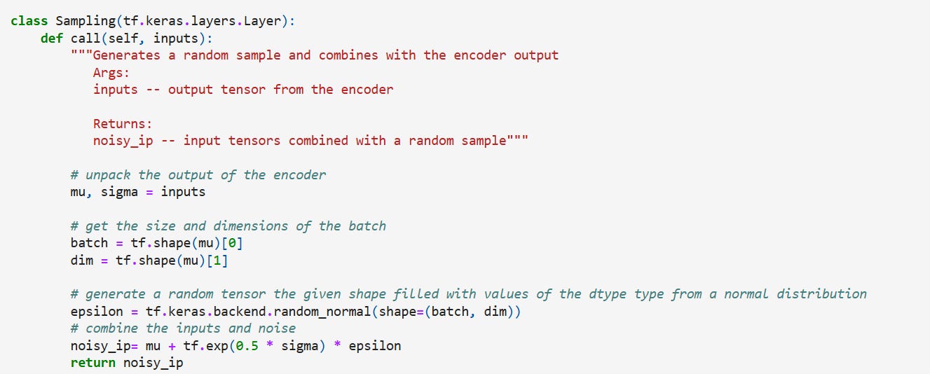
Sampling
We will begin by building the sampling class which is the bottleneck of the network. This will provide the Gaussian noise input along with the mean and standard deviation of the encoder's output. The output of this layer is given by the equation,
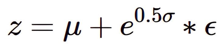
where μ = mean, σ = standard deviation, and ϵ = random sample
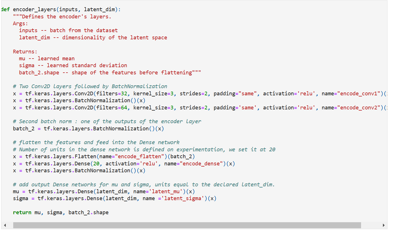
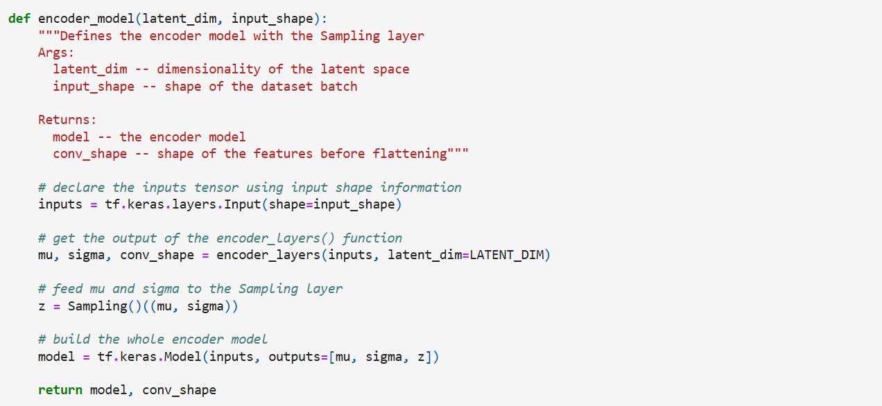
Let’s build the encoder now. For the sake of convenience, while constructing the decoder, we will also output the shape of features before flattening it. The encoder is built as shown below,
Coding it up,
And putting it together with the sampling class,
Decoder
The decoder expands the latent representations back to the original image dimensions. We’ve used a dense layer with batch normalization, two transpose convolution layers, and a single transpose convolution layer with 1 filter to bring it back to the original shape as the input.
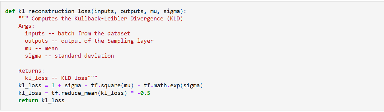
Loss functions
In VAEs, we calculate two losses,
Reconstruction loss: Just like autoencoders, we want to find the difference between the input and the decoder output. So, similar to autoencoders, we use a metric like MSE to calculate the difference between input and decoder output. In our case, we are using Binary Cross-Entropy.
KL divergence loss: The math and reasoning behind this are explained in the separate article linked earlier. This also acts as regularizer and prevents the model from encoding too much information (and making it work like an autoencoder
The combined VAE loss is a weighted sum of the Reconstructed and KL divergence losses.
We’ll define a function for KL divergence loss, reconstruction loss while be including in the training loop.
Finally, lets put everything together and create the VAE model
Note: Loss computation doesn’t use y_true and y_pred so it can’t be used in model.compile()
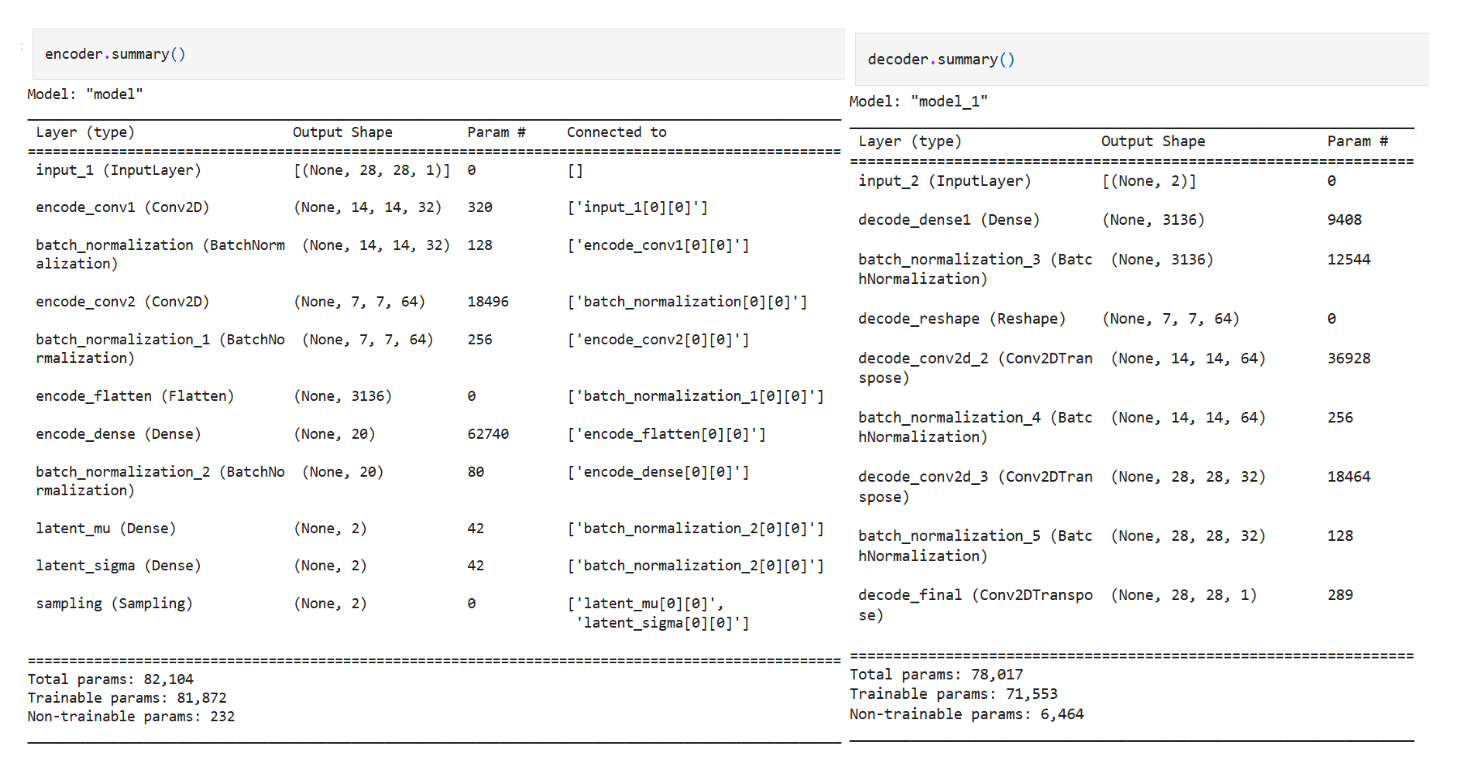
The model summary for encoder and decoder looks like this,
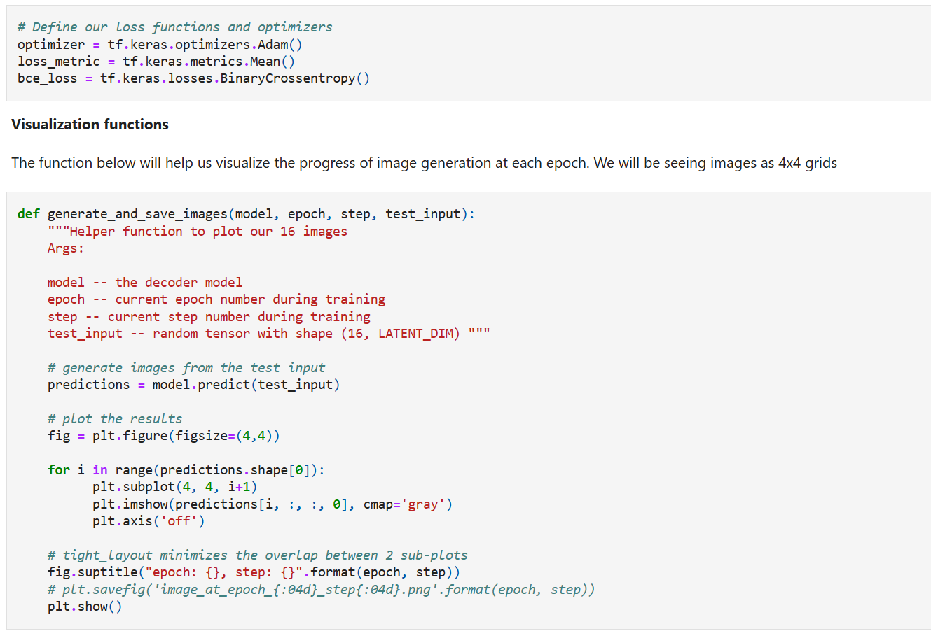
Model training
Here we define the reconstruction loss, optimizer, and metric followed by a visualization function to help us visualize the progress of image generation at each epoch. We will be seeing images as 4x4 grids.
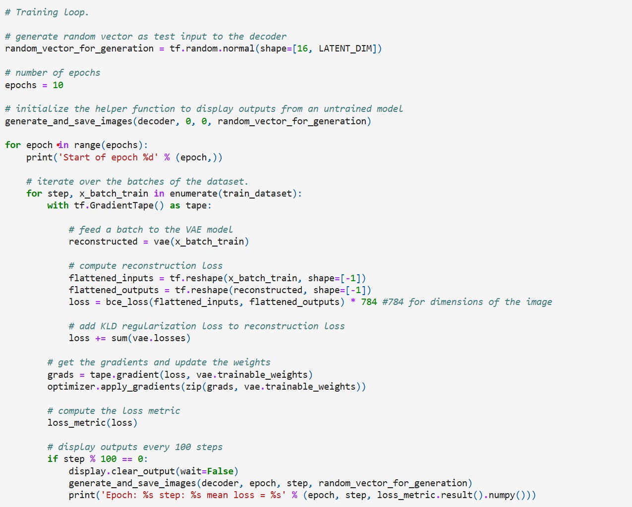
Training Loop
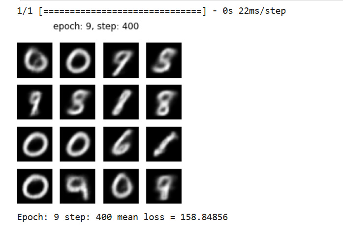
We will run the training for 10 epochs for now and display the generated images at each epoch. As the network learns and we will see images that resemble the MNIST dataset.
We just run the model for 10 epochs (don’t do this if you are building an actual VAE model!) and the results look like this,
REFERENCES
Deep dive into Autoencoders and VAE: https://towardsdatascience.com/understanding-variational-autoencoders-vaes-f70510919f73
Image generation with VAE: https://www.machinelearningnuggets.com/how-to-generate-images-with-variational-autoencoders-vae-and-keras/
Mathematics for Bayesian Networks – Part 1, Introducing the Basic Terminologies in Probability and Statistics: https://mohanarc.substack.com/p/mathematics-for-bayesian-networks
Mathematics for Bayesian Networks – Part 2, Introduction to Bayes Theorem: https://mohanarc.substack.com/p/mathematics-for-bayesian-networks-3d1
Mathematics for Bayesian Networks – Part 3, Advanced Concepts and Examples: https://mohanarc.substack.com/p/mathematics-for-bayesian-networks-943
Mathematics for Bayesian Networks – Part 4, Distributions beyond the “Normal” : https://mohanarc.substack.com/p/mathematics-for-bayesian-networks-103
ELBO and KL divergence: https://open.substack.com/pub/mohanarc/p/applications-of-bayes-theorem-kl?r=1ljeoy&utm_campaign=post&utm_medium=web